The latest version of this document will always be found here.
Note that this is an extremely brief and limited introduction to R, with the examples writ with the UC Irvine BDUC system in mind. There are many more complete introductory docs, some of the best listed in the section below. This is only to get your toes wet.
|
|
Some assumptions
The following tutorial assumes that you’re using a Linux system from the bash shell, you’re familiar navigating directories on a Linux system using cd, using the basic shell utilities such as head, tail, less, and grep, and the minimum R system has been installed on your system. If not, you should peruse a basic introduction to the bash shell. The bash prompt is shown as bash %. The R shell prompt is > and R commands will be prefixed by the > to denote it. Inline comments are prefixed by and can be copied into your shell along with the R or bash commands they comment - the shields them from being executed, but do NOT copy in the R or bash shell prompt. For a quick introduction to basic data manipulation with Linux, please refer to the imaginatively named Manipulating Data on Linux. |
1. R’s operational modes
R is a programming language designed explicitly for statistical computation. As such, it has many of the characteristics of a general-purpose language including iterators, control loops, network and database operations, many of which are useful, but in general not as easy to use as the more general Python or Perl
R can operate in 2 modes, as an interactive interpreter (the R shell) and as a scripting language, much like Perl or Python. Typically the R shell is used to try things out and the serial commands written in the R language and saved in a file are used to automate operations once the sequence is well-defined and debugged.
While it is not a great language for procedural programming, it does excel at mathematical and statistical manipulations. However, it does so in an odd way, especially for those who have done procedural programming before. R is quite object-oriented in that you tend to deal with data objects rather than with individual integers, floats, arrays, etc. The best way to think of data if you have programmed in C is to think of R data (typically termed tables or frames) as C structs, arbitrary constructs that can be dealt with by name. If you haven’t programmed in a procedural language, it may actually be easier for you. R manipulates chunks of data similar to how you might think of them. For example, "multiply that column by 3.54" or "pivot that spreadsheet".
For a still-brief but more complete overview of R, see Wikipedia’s entry for R.
2. Graphics and Graphical User Interfaces for R
R was developed as a commandline language. However, it has gained progressively more graphics capabilities and graphical user interfaces (GUIs). Some notable examples are the de facto standard R GUI R Commander, the elegant and powerful interactive graphics utility ggobi, and the fully graphical statistics package gretl which was developed external to R for time-series econometrics but which now supports R as an external module.
In addition, many routines in R are packaged with their own GUIs so that when called from the commandline interface, the GUI will pop up and allow the user to interact with a mouse rather than the keyboard.
As opposed to fully integrated commercial applications which have a cohesive interface, these packages differ slightly in the way that they approach getting things done, but in general the mechanisms follow generally accepted user interface conventions.
3. Getting help on R
After starting R, you can usually start R’s internal help with:
bash %  R  # more comments on R's startup state below
# R startup messages deleted
> help.start().
This will start a browser page with a lot of links to R documentation, both introductory and advanced.
If that help is not installed, most R help can be found in PDF and HTML at the R documentation page.
There is a very useful 100 page PDF book called: An Introduction to R (also in HTML). Especially note Chapter 1 and Appendix A on page 78, which is a more sophisticated, (but less gentle) tutorial than this.
Note also that if you have experience in SAS or SPSS, there is a good introduction written especially with this experience in mind. It has been expanded into a large book (to be released imminently), but much of the core is still available for free as R for SAS and SPSS Users
There is another nice Web page that provides a quick, broad intro to R appropriately called Using R for psychological research: A simple guide to an elegant package which manages to compress a great deal of what you need to know about R into about 30 screens of well-cross-linked HTML.
There is also a website that expands on simple tutorials and examples, so after buzzing thru this very simple example, please continue to the QuickR website
Thomas Girke at UC Riverside has a very nice HTML Introduction to R and Bioconductor as part of his Bioinformatics Core, which also runs frequent R-related courses which may be of interest for the Southern California area.
4. Start the R interpreter
On the BDUC cluster, we host several versions of R. You if you want a particular version, you’ll have to specify it via the module command:
bash % module load R/2.12.2
which causes the module info to be spat out and then you can start R with:
bash % R # simple, no?
# if you get the line shown below:
[Previously saved workspace restored]
you had saved the previous data environment and if you type ls() you’ll see all the previously created variables:
> ls()
 [1] "aa"          "data.matrix" "fil_ss"      "i"           "ma5"
 [6] "mn"          "mn_tss"      "norm.data"   "sg5"         "ss"
[11] "ss_mn"       "sss"         "tss"         "t_ss"        "tss_mn"
[16] "x"
If the previous session was not saved, there will be no saved variables in the environment
> ls()
character(0) # denotes an empty character (= nothing there)
NB: In many cases the data objects can be manipulated as you would files in the Unix shell, with the takes-some-getting-used-to of adding the almost-always-required parens afterwards:
> ls() # lists all data objects in view
> ls(someframe) # may give additional inforamtion on the frame
> rm(someframe) # deletes the 'someframe' data object
To determine what an object is, you can use a variety of methods, but one of the most useful is str (get the structure of an abject).
> str(aa)  # aa is a table or data.frame resulting from reading in a 25MB file.
'data.frame':   385238 obs. of  6 variables:
 $ ID    : Factor w/ 1649 levels "ENSXETG00000000007_SCAFFOLD_1356_47264_67263",..: 1 1 1 1 1 1 1 1 1 1 ...
 $ BEGIN : int  1 70 139 232 301 370 439 508 577 658 ...
 $ END   : int  50 119 188 281 350 419 488 557 626 707 ...
 $ Blue  : num  -0.67 -0.47 0.36 0.42 0.09 0.22 -0.42 0.61 0.71 1.61 ...
 $ Red   : num  2.8 2.56 2.96 -0.76 -2.6 -1.52 -0.36 -3.24 -1.8 -3.36 ...
 $ RedNeg: num  -0.7 -0.64 -0.74 0.19 0.65 0.38 0.09 0.81 0.45 0.84 ...

> str(y) # y is a vector of size 50
 num [1:50] -0.202 -0.418  0.325 -0.377 -0.405 ...
You can also use dim() to get the bare dimensions of the data structure. Always a good idea before you try to view it by referencing the data directly without limits.
> dim (aa)  # aa is a table or data.frame resulting from reading in a 25MB file.
[1] 385238      6
And to address the individual vectors composing the structure, just use the form Structure$Vector.
ie: aa$Blue refers to the structure aa, vector Blue (see above).
Getting the size of objects
You can also obtain the actual byte-size of the objects in memory via:
# if ls() gives you the following:
> ls ()
 [1] "d"          "e"          "eset"       "eSet"       "gset"
 [6] "gset_wgcna" "gset60862"  "idx"        "o"          "pd60862"
[11] "pheno"

# then you can list the RAM-resident sizes via:
> for (thing in ls()) { message(thing); print(object.size(get(thing)), units='auto') }
d
63.4 Kb
e
153.4 Mb
eset
96.6 Mb
eSet
6.2 Mb
gset
96.6 Mb
gset_wgcna
153.4 Mb
gset60862
7.6 Mb
idx
48 bytes
o
63.4 Kb
pd60862
4 Mb
pheno
129.5 Kb
5. Some basic R data types
Before we get too far, note that R has a variety of data structures that may be required for different functions.
Some of the main ones are:
-
numeric - (aka double) the default double-precision (64bit) float representation for a number.
-
integer - a single-precision (32bit) integer.
-
single - a single precision (32bit) float
-
string - any character string ("harry", "r824_09_hust", "888764"). Note the last is a number defined as a string so you couldn’t add "888764" + 765.
-
vector - a series of data types of the same type. (3, 5, 6, 2, 15) is a vector of numerics. ("have", "third", "start", "grep) is a vector of strings.
-
matrix - an array of identical data types - all numerics, all strings, all booleans, etc.
-
data.frame - a table (another name for it) or array of mixed data types. A column of strings, a column of integers, a column of booleans, 3 columns of numerics.
-
list - a concatenated series of data objects.
6. Loading data into R
This process is described in much more detail in the document R Data Import/Export, but this will give you a short example of one of the most popular ways of loading data into R.
The following reads the example data file above (red+blue_all.txt) into an R table called aa; note the ,header=TRUE option which uses the file header line to name the columns. In order for this to work, the column headers have to be separated by the same delimiter as the data (usually a space or a tab).
> aa <- read.table(file="red+blue_all.txt",header=TRUE) # try it
I have run into situations where read.table() would simply not read in a file which I had validated with an external Perl script:
> em <- read.table(file="long_complicated_data_file",header=TRUE,sep="\t",comment.char="#") # try it
Error in scan(file, what, nmax, sep, dec, quote, skip, nlines, na.strings,  :
  line 134 did not have 29 elements
In these cases, using read.delim() may be more successful:
em <- read.delim(file="long_complicated_data_file",na.strings = "", fill=TRUE, header=T, sep="\t")
>
(see also Thomas Girke’s excellent R/BioC Guide.)
Note that in R, you can work left to right or right to left, altho the left pointing arrow is the usual syntax. The above command could also have been given as :
> read.table(file="red+blue_all.txt",header=TRUE) -> aa # try it
Did we get the col names labeled correctly?
> names(aa)  # try it
[1] "ID"    "BEGIN" "END"   "Blue"  "Red"
Many functions will require the data as a matrix (a data structure whose components are identical data types, usually strings. The following will load the file into a matrix, doing the conversions along the way. This command also shows the use of the sep="\t" option which explicitly sets the data delimiter to the TAB character.
Data <- as.matrix(read.table("red+blue_all.txt", sep="\t", header=TRUE))
7. Viewing data
To view some of the table, we only need to reference it. R assumes that a naked variable is a request to view it. An R table is referenced in [rows,column] order. That is, the index is [row indices, col indices], so that a reference like aa[1:6,1:5] will show a square window of the table; rows 1-6, columns 1-5
Also: R parameters are 1-indexed, not 0-indexed, tho it seems pretty forgiving (if you ask for [0-6,0-5], R will assume you meant [1-6,1-5]. also note that R requires acknowledging that the data structures are n-dimensional: to see rows 1-11, you can’t just type:
> aa[1:11] # try it!
but must instead type:
> aa[1:11,] # another dimension implied by the ','
To slice the table even further, you can view only those elements that interest you
  # R will provide row and column headers if they were provided.
  # if they weren't provided, it will provide column indices.
> aa[3:12,4:5]  # try it.
8. Using HDF5 files with R
HDF5 (see also the Wikipedia entry) is a very sophisticated format for data which is being used increasingly in domains that were not previously using it, chiefly in Financial Record Archiving, and Bioinformatics.
As the name suggests, internally, it is a hierarchically organized hyperslab, a structure of multi-dimensional arrays of the same data type (ints, floats, bools, etc), sort of like the file equivalent of a C struct. There can be multiple different such arrays but each contains data of the same type.
R supports reading and writing HDF5 files with the rhdf5 library, among others.
8.1. Reading HDF5 files into R
If you are only going to be reading HDF5 files provided by others, the approach is very easy:
# assuming the rhdf5 library is installed
> library(rhdf5)
> h5 <- h5read("SVM_noaa_ops.h5")  # a 12MB HDF5 file
> h5ls("SVM_noaa_ops.h5")         # describe the structure of the HDF5 file
                         group                  name       otype    dclass
0                            /              All_Data   H5I_GROUP
1                    /All_Data      VIIRS-M1-SDR_All   H5I_GROUP
2   /All_Data/VIIRS-M1-SDR_All              ModeGran H5I_DATASET   INTEGER
3   /All_Data/VIIRS-M1-SDR_All              ModeScan H5I_DATASET   INTEGER
4   /All_Data/VIIRS-M1-SDR_All  NumberOfBadChecksums H5I_DATASET   INTEGER
5   /All_Data/VIIRS-M1-SDR_All NumberOfDiscardedPkts H5I_DATASET   INTEGER
6   /All_Data/VIIRS-M1-SDR_All   NumberOfMissingPkts H5I_DATASET   INTEGER
7   /All_Data/VIIRS-M1-SDR_All         NumberOfScans H5I_DATASET   INTEGER
8   /All_Data/VIIRS-M1-SDR_All              PadByte1 H5I_DATASET   INTEGER
9   /All_Data/VIIRS-M1-SDR_All     QF1_VIIRSMBANDSDR H5I_DATASET   INTEGER
10  /All_Data/VIIRS-M1-SDR_All          QF2_SCAN_SDR H5I_DATASET   INTEGER
11  /All_Data/VIIRS-M1-SDR_All          QF3_SCAN_RDR H5I_DATASET   INTEGER
12  /All_Data/VIIRS-M1-SDR_All          QF4_SCAN_SDR H5I_DATASET   INTEGER
13  /All_Data/VIIRS-M1-SDR_All  QF5_GRAN_BADDETECTOR H5I_DATASET   INTEGER
14  /All_Data/VIIRS-M1-SDR_All              Radiance H5I_DATASET   INTEGER
15  /All_Data/VIIRS-M1-SDR_All       RadianceFactors H5I_DATASET     FLOAT
16  /All_Data/VIIRS-M1-SDR_All           Reflectance H5I_DATASET   INTEGER
17  /All_Data/VIIRS-M1-SDR_All    ReflectanceFactors H5I_DATASET     FLOAT
18                           /         Data_Products   H5I_GROUP
19              /Data_Products          VIIRS-M1-SDR   H5I_GROUP
20 /Data_Products/VIIRS-M1-SDR     VIIRS-M1-SDR_Aggr H5I_DATASET REFERENCE
21 /Data_Products/VIIRS-M1-SDR   VIIRS-M1-SDR_Gran_0 H5I_DATASET REFERENCE
          dim
0
1
2           1
3          48
4          48
5          48
6          48
7           1
8           3
9  3200 x 768
10         48
11         48
12        768
13         16
14 3200 x 768
15          2
16 3200 x 768
17          2
18
19
20         16
21         16

# in a slightly different format, 'h5dump' provides similar information:
> h5dump(file="SVM_noaa_ops.h5", load=FALSE)
$All_Data
$All_Data$`VIIRS-M1-SDR_All`
$All_Data$`VIIRS-M1-SDR_All`$ModeGran
  group     name       otype  dclass dim
1     / ModeGran H5I_DATASET INTEGER   1

$All_Data$`VIIRS-M1-SDR_All`$ModeScan
  group     name       otype  dclass dim
1     / ModeScan H5I_DATASET INTEGER  48

 ... <etc>
Other R data manipulations are fairly easy as well.
# you can read parts of the HDF5 hyperslab into an R variable as well
# the following reads a subgroup into an R object
> h5_aa <- h5read("SVM_noaa_ops.h5", "/All_Data/VIIRS-M1-SDR_All")

# and this is what h5_aa contains.
> names(h5_aa)
 [1] "ModeGran"              "ModeScan"              "NumberOfBadChecksums"
 [4] "NumberOfDiscardedPkts" "NumberOfMissingPkts"   "NumberOfScans"
 [7] "PadByte1"              "QF1_VIIRSMBANDSDR"     "QF2_SCAN_SDR"
[10] "QF3_SCAN_RDR"          "QF4_SCAN_SDR"          "QF5_GRAN_BADDETECTOR"
[13] "Radiance"              "RadianceFactors"       "Reflectance"
[16] "ReflectanceFactors"

# see each sub-object by referencing it in the standard R way:
> h5_aa$NumberOfScans
[1] 48
8.2. Writing HDF5 files from R
Writing HDF5 files is slightly more difficult, but only because you have to be careful that you’re writing to the right group and that there is congruence between R and HDF5 data types and attributes. The rhdf5 docs have good examples for this.
9. Visualizing Data with ggobi
While there are many ways in R to plot your data, one unique benefit that R provides is its interface to ggobi, an advanced visualization tool for multivariate data, which for the sake of argument is more than 3 variables.
10. Operations on Data
To operate on a column, ie: to multiply it by some value, you only need to reference the column ID, not each element. This is a key idea behind R’s object-oriented approach. The following multiplies the column Red of the table aa by -1 and stores the result in the column 'RedNeg. There’s no need to pre-define the RedNeg column; R will allocate space for it as needed.
> aa$RedNeg = aa$Red * -1   # try it

# the table now has a new column called 'RedNeg'
> aa[1:4,]      # try it
If you want to have the col overwritten by the new value, simply use the original col name as the left-hand value. You can also combine statements by separating them with a ;
> aa$Red = aa$Red * -2; aa[1:4,] # mul aa$Red by -2 and print the 1st 4 lines
To transpose (aka pivot) a table:
> aacopy <- aa # copy the table

> aac_t <- t(aacopy) # transpose the table

# show the all the rows & 1st 3 columns of the transposed table
> aac_t[,1:3]
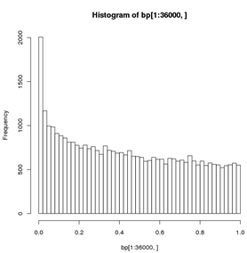
To bin a vector and visualize the binning:
> bp <- read.table(file="just.bayesp",header=TRUE) # 36K fp values
> hist(bp[1:36000,],breaks=50,plot="True")
# see result below
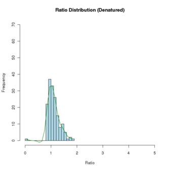
To draw a histogram of a data vector and spline the distribution curve, using the file MS21_Denat_C_Native_E.txt
# read the file into a dataframe
$ cat MS21_Denat_C_Native_E.txt
Denat   Native
1.83    4.80
1.78    3.95
1.75    3.72
1.61    3.60
1.60    3.32
 ...
# start R
$ R

> bth <- read.table(file="MS21_Denat_C_Native_E.txt",header=TRUE,sep="\t",comment.char="#")
Check it
> str(bth)
'data.frame':   233 obs. of  2 variables:
 $ Denat : num  1.83 1.78 1.75 1.61 1.6 1.6 1.58 1.55 1.51 1.5 ...
 $ Native: num  4.8 3.95 3.72 3.6 3.32 3.23 3.1 2.9 2.7 2.66 ...

# Create a histogram for the 'Denat' column.  The following cmd not only plots the histogram
# but also populates the 'hhde' histogram object.
# breaks =  how many bins there should be (controls the size of the bins
# plot = to plot or not to plot
# labels = if T, each bar is labeled with the numeric value
# main, xlab, ylab = plot title, axis labels
# col = color of hist bars
# ylim, xlim = axis limits; this was set to allow another histogram to fit inside
#  the defined limits; if not set, the limits will be those of the data.

> hhde <-hist(bth$Denat,breaks=16,plot="True",labels=F, main="Ratio Distribution (Denatured)",xlab="Ratio",ylab="Frequency", col="lightblue",ylim=c(0,70), xlim=c(0,5) )

# now plot a smoothed distribution using the hhde$mids (x) and hhde$counts (y)
# df = degrees of freedom, how much smoothing is applied;
#    (how closely the line will follow the values)
> lines(sm.spline(hhde$mids,hhde$counts, df=10), lty=1, col = "green")
11. Exporting Data
Ok, you’ve imported your data, analyzed it, generated some nice plots and dataframes. How do you export it to a file so it can be read by other applications? As you might expect, R provides some excellent documentation for this as well. The previously noted document R Data Import/Export describes it well. It’s definitely worthwhile reading it in full, but the very short version is that the most frequently used export function is to write dataframes into tabular files, essentially the reverse of reading Excel spreadsheets, b ut in text form. For this, we most often use the write.table() function. Using the aa dataframe already created, let’s output some of it:
> aa[1:3,] # lets see what it looks like 'raw'
                                            ID BEGIN END  Blue  Red
1 ENSXETG00000000007_SCAFFOLD_1356_47264_67263     1  50 -0.67 0.70
2 ENSXETG00000000007_SCAFFOLD_1356_47264_67263    70 119 -0.47 0.64
3 ENSXETG00000000007_SCAFFOLD_1356_47264_67263   139 188  0.36 0.74

> write.table(aa[1:3,])
"ID" "BEGIN" "END" "Blue" "Red"
"1" "ENSXETG00000000007_SCAFFOLD_1356_47264_67263" 1 50 -0.67 0.7
"2" "ENSXETG00000000007_SCAFFOLD_1356_47264_67263" 70 119 -0.47 0.64
"3" "ENSXETG00000000007_SCAFFOLD_1356_47264_67263" 139 188 0.36 0.74

# in the write.table() format above, it's subtly different.  Note the quoting and spacing.
# You can address all these in the various arguments to write.table(), for example:

> write.table(aa[1:3,], quote = FALSE, sep = "\t",row.names = FALSE,col.names = TRUE)
ID      BEGIN   END     Blue    Red
ENSXETG00000000007_SCAFFOLD_1356_47264_67263    1       50      -0.67   0.7
ENSXETG00000000007_SCAFFOLD_1356_47264_67263    70      119     -0.47   0.64
ENSXETG00000000007_SCAFFOLD_1356_47264_67263    139     188     0.36    0.74

# note that I omitted a file specification to dump the output to the screen.  To send
# the same output to a file, you just have to specify it:

> write.table(aa[1:3,], file="/path/to/the/file.txt", quote = FALSE, sep = "\t",row.names = FALSE,col.names = TRUE)


# play around with the arguments, reversing or modifying the argument values.
# the entire documentation for write.table is available from the commandline with
# '?write.table'
12. Basic Statistics
Now, let’s get some basic descriptive stats out of the original table. 1st, load the lib that has the functions we’ll need
> library(pastecs)  # load the lib that has the correct functions
> attach(aa) # make the Red & Blue columns usable as variables.

# following line combines an R data structure by column.
# type 'help(cbind)' or '?cbind' for more info on cbind, rbind

> redblue <- cbind(Red,Blue)

# the following calculates a table of descriptive stats for both the Red & Blue variables
> stat.desc(redblue)
                       Red          Blue
nbr.val       3.852380e+05  3.852380e+05
nbr.null      2.486000e+03  2.188000e+03
nbr.na        0.000000e+00  0.000000e+00
min          -1.504000e+01 -5.130000e+00
max           2.256000e+01  5.340000e+00
range         3.760000e+01  1.047000e+01
sum          -6.929548e+04  3.060450e+03
median        4.000000e-02  0.000000e+00
mean         -1.798771e-01  7.944310e-03
SE.mean       3.826047e-03  1.115451e-03
CI.mean.0.95  7.498938e-03  2.186250e-03
var           5.639358e+00  4.793247e-01
std.dev       2.374733e+00  6.923328e-01
coef.var     -1.320198e+01  8.714826e+01
You can also feed column numbers to stat.desc to generate similar results:
stat.desc(some_table[2:13])
             stress_ko_n1 stress_ko_n2 stress_ko_n3 stress_wt_n1 stress_wt_n2
nbr.val      3.555700e+04 3.555700e+04 3.555700e+04 3.555700e+04 3.555700e+04
nbr.null     0.000000e+00 0.000000e+00 0.000000e+00 0.000000e+00 0.000000e+00
nbr.na       0.000000e+00 0.000000e+00 0.000000e+00 0.000000e+00 0.000000e+00
min          1.013390e-04 1.041508e-04 1.003806e-04 1.013399e-04 1.014944e-04
max          2.729166e+04 2.704107e+04 2.697153e+04 2.664553e+04 2.650478e+04
range        2.729166e+04 2.704107e+04 2.697153e+04 2.664553e+04 2.650478e+04
sum          3.036592e+07 2.995104e+07 2.977157e+07 3.054361e+07 3.055979e+07
median       2.408813e+02 2.540591e+02 2.377578e+02 2.396799e+02 2.382967e+02
mean         8.540068e+02 8.423388e+02 8.372915e+02 8.590042e+02 8.594593e+02
SE.mean      8.750202e+00 8.608451e+00 8.599943e+00 8.810000e+00 8.711472e+00
CI.mean.0.95 1.715066e+01 1.687283e+01 1.685615e+01 1.726787e+01 1.707475e+01
var          2.722458e+06 2.634967e+06 2.629761e+06 2.759796e+06 2.698411e+06
std.dev      1.649987e+03 1.623258e+03 1.621654e+03 1.661263e+03 1.642684e+03
coef.var     1.932054e+00 1.927085e+00 1.936785e+00 1.933941e+00 1.911300e+00

<etc>
There is also a basic function called summary, which will give summary stats on all components of a dataframe.
> summary(aa)
                                               ID             BEGIN
 ENSXETG00000004313_SCAFFOLD_317_890727_910726  :   289   Min.   :    1
 ENSXETG00000010135_SCAFFOLD_646_44207_64206    :   289   1st Qu.: 4875
 ENSXETG00000017293_SCAFFOLD_132_1100669_1120668:   289   Median : 9722
 ENSXETG00000020596_SCAFFOLD_474_677230_697229  :   289   Mean   : 9781
 ENSXETG00000021861_SCAFFOLD_101_1701655_1721654:   289   3rd Qu.:14639
 ENSXETG00000023499_SCAFFOLD_486_295358_315357  :   289   Max.   :19950
 (Other)                                        :383504
      END             Blue                Red               RedNeg
 Min.   :   50   Min.   :-5.130000   Min.   :-15.0400   Min.   :-5.64000
 1st Qu.: 4924   1st Qu.:-0.470000   1st Qu.: -1.7600   1st Qu.:-0.39000
 Median : 9771   Median : 0.000000   Median :  0.0400   Median :-0.01000
 Mean   : 9830   Mean   : 0.007944   Mean   : -0.1799   Mean   : 0.04497
 3rd Qu.:14688   3rd Qu.: 0.480000   3rd Qu.:  1.5600   3rd Qu.: 0.44000
 Max.   :19999   Max.   : 5.340000   Max.   : 22.5600   Max.   : 3.76000
13. The commercial Revolution R is free to Academics
Recently a company called Revolution Analytics has started to commercialize R, smoothing off the rough edges, providing a GUI, improving the memory management, speeding up some core routines. If you’re interested in it, you can download it from here.