Big Data for Biologists

1. The Problem with Digital Biology

Since the transition to genomics, data has gotten larger and larger.

Growth of Genbank

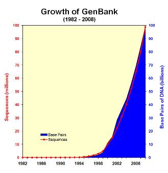
Fortunately, until the mid-90’s, disk size, network bandwidth & CPU speeds were increasing much faster so everyone was pretty happy. Now with HTS, some bottlenecks are starting to crop up.

Moore’s Law predicts that CPU power increases by 60% per year, but CPU clock speeds are essentially static and computational power is now being increased by multicore CPUs and GPUs which require considerably different programming techniques.

Network speeds are fairly fast, but are not increasing very fast locally because copper is reaching its upper limit and even if it increases a few more steps it will be at very short distances. Optical networks hold huge promise, but the technology is comparatively expensive and tempermental.

Disk capacity is continuing to increase exponentially as well, but large RAIDs are starting to approach the Uncorrectable Bit Error Rate problem and so the amount of data that we can store in contiguous devices is starting to hit a limit. And if you want that data backed up, the problem/expense doubles.

So what do we do? Learn to live with it.

If you don’t learn to use the commandline, you’ll be 1-3 years behind the cutting edge of any computer-aided analysis. Building good User Interfaces are hard. Building good commercial ones are even harder.

Example of a commandline to search human chromosome 1 (254MB) for a pattern with one degeneracy and extract the match plus flanking sequence:

time tacg -S -p bubba,gtgaggacttaga,1 -X 22,22,1 <chr1.fa >out
real    0m27.448s
user    0m19.105s
sys     0m1.312s
(9.4 MB/s)

For many analytical tools there simply are no GUI equivalents.

For a good introduction to Linux and the bash shell, spend a a few hours with Software Carpentry

2. How much Data can you afford?

It really boils down to the question above.

What is the minimum data you need to keep around?
Do you really need to back up everything?
Where do you put this data?
- on large RAIDs, preferably RAID6 (any OS) or ZFS (Solaris only) or be prepared to give a LOT of money to BlueArc, Isilon, NetApp, EMC, Sun, IBM, etc.
- Open Source Parallel File systems are starting to be reliable enough to use in production as well (Lustre, PVFS, Gluster, etc)
- if on your Desktop, use reliable disks & RAID them if possible.
How do you move this data?
- As much as possible, don’t. And if you can, use rsync (elegant incremental copy),
- for full copies, use bbcp or fdt.
- see How to transfer large amounts of data via network.

Note that for most HTS data, using encryption is not ncessary (do you care if someone intercepts your short-read file?) so for most files, don’t bother with encryption. On the other hand, compression can help a lot on slower connections (plaintext sequence data is compressible to 1/4 to 1/3 the uncompressed size.

100Mb network --→ ~10MB/s
1Gb network --→ ~80MB/s

so 200GB of files → ~45min over a 1Gb net if the storage can handle that speed.

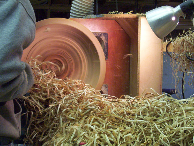
A somewhat wooden analogy

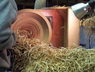
The above image of a spinning wooden dish on a lathe is a (strained) analogy to a disk drive. The faster the dish spins, the more wood (data) can be scraped off it per second; the closer to the outside, the more wood (data) can be scraped off per second. If you have multiple lathes (disks), each additional lathe increases the amount of wood (data) that can be scraped off per second.

3. Not all Big Data is the same

There is hope, especially for some types of data.

3.1. Types of data

3.1.1. Plaintext

ASCII plaintext vs binary vs MS Word doc format For editing plaintext files, use a plaintext editor, such as Notepad for Windows or Jedit (excellent, for all platforms).
Mac and Linux plaintext now use the same end-of-line character (line feed; \n); Windows is still different (carriage return + line feed; \r\n)

3.1.2. Structured Text

XML (like HTML) Example
FASTA
FASTQ
Protein Data Bank
Other Structural formats

3.1.3. Binary

images
compressed data
executables, object files, libraries
specially constructed application-specific data.

3.1.4. Databases

flatfile (FASTA sequences)
relational (MySQL, PostgreSQL)
key:value type DBs (color:red, fruit:bananas)

3.1.5. Self-describing Data

Structured (strided, self-describing) binary files (such as NetCDF, HDF5, & BioHDF).

Self-describing Data Formats are a special case of data file and one that holds great promise for large Biological data. It has been used for many kinds of large data for more than a decade in the Physical Sciences and since part of Biology is now transitioning to a Physical Science, it becomes appropriate to use their proven approaches.

These types of files:

can represent N-dimensional data
have unlimited extents (such as open-ended time series)
are internally like an entire filesystem, so groups of related data can be bundled together.
are indexed (or strided) so that offsets to a particular piece of data can be found very quickly (microseconds).
are dynamically ranged so the file uses only as many bits to represent a range of data as it really needs. ('int’s can be represented as bits, depending on the data range)

The BioHDF project is already starting to use this approach, specifically for representing HTS data and we should start seeing code support later this year. It happens that Charlie Zender (author of nco, a popular utility suite for manipulating NetCDF files) is in UCI’s ESS dept.

There is another technology that has been used quite successfully in the Climate Modelling field which is the OpenDAP Server. This software keeps the data on a central server and allows researchers to query it to return various chunks of data and to transform them in various ways. In some ways it’s very much like a web server such as the UCSC Genome Center’s Browser system, but it allows much more computationally heavy transforms.

4. Some useful tools

4.1. Basic utilities

Mac OSX is fine (based on Unix). The OS and UI are fairly stable.

Linux is best (re-written Unix). The OS and UI are fairly stable.

Windows is a strange bastard hybrid system designed to transport dollars from your wallet to Microsoft that also makes writing software very difficult. Every other year Microsoft replaces the system that you’ve learned to tolerate with one that bears little similarity to it and charges you for that loss of productivity.

But most damning for research is that it makes it hard to write portable software.

If you want an amusing read on the development of the Mac, Linux and Windows, Neal Stephenson has a great (if long) take on it called In the Beginning was the Command Line

The following are basic Linux utilities.

4.1.1. ls

ls lists the files in a directory

4.1.2. grep

grep (and relatives egrep, fgrep, agrep, nrgrep) searches for regular expressions in files. A regular expression (aka regex) is very powerful pattern matching approach. Read THE regex book here.

4.1.3. head & tail

head shows you the top of a file. tail shows you the bottom of the file.

4.1.4. cut, scut & cols

cut and scut let you slice out and re-arrange columns in a file, spearated by a defined delimiter. cols lines up those files so you can make sense of them.

These and more such utilities are discussed at much greater length in Manipulating Data on Linux.

4.2. Applications on the BDUC Cluster

*R/2.10.0          *gaussian/3.0       *mosaik/1.0.1388     readline/5.2
*R/2.11.0           gnuplot/4.2.4       mpich/1.2.7        *samtools/0.1.7
*R/2.8.0           *gromacs_d/4.0.7     mpich2/1.1.1p1      scilab/5.1.1
*R/dev             *gromacs_s/4.0.7    *msort/20081208      sge/6.2
*abyss/1.1.2        hadoop/0.20.1      *namd/2.6           *soap/2.20
 antlr/2.7.6        hdf5-devel/1.8.0   *namd/2.7b1          sparsehash/1.6
*autodock/4.2.3     hdf5/1.8.0          ncl/5.1.1           sqlite/3.6.22
*bedtools/2.6.1     imagej/1.41         nco/3.9.6           subversion/1.6.9
*bfast/0.6.3c       interviews/17       netCDF/3.6.3       *sva/1.02
 boost/1.410        java/1.6            neuron/7.0         *tacg/4.5.1
*bowtie/0.12.3     *maq/0.7.1          *nmica/0.8.0         tcl/8.5.5
*bwa/0.5.7          matlab/R2008b       octave/3.2.0        tk/8.5.5
*cufflinks/0.8.1    matlab/R2009b       open64/4.2.3       *tophat/1.0.13
 fsl/4.1           *mgltools/1.5.4      openmpi/1.4        *triton/4.0.0
*gapcloser         *modeller/9v7        python/2.6.1        visit/1.11.2

* of possible interest to Biologists.

example:

$ module load abyss

ABySS - assemble short reads into contigs
See: /apps/abyss/1.1.2/share/doc/abyss/README
or 'ABYSS --help'
or 'man /apps/abyss/1.1.2/share/man/man1/ABYSS.1'
or 'man /apps/abyss/1.1.2/share/man/man1/abyss-pe.1'

Also, ClustalW2/X, SATE (including MAFFT, MUSCLE, OPAL, PRANK, RAxML), readseq, phylip, etc.

4.3. Other Genomic Visualization Tools

Some other Genomic Visualization tools are listed here. (Some of them are installed on BDUC; some are web tools; some still need to be installed.

5. Which programming language is best for Biology?

Sometimes what you need to do just isn’t handled by an existing utility and you need to write it yourself. For those situations which call on data mangling/massaging, I’d recommend either Perl & BioPerl (or Python & BioPython).

Perl has an elegant syntax for handling much of the simple line-based data mangling you might run into:

#!/usr/bin/perl -w
while (<>) {          # while there's still more lines to process
   chomp;             # chew off the 'newline' character
   $N = @L = split;   # split all the columns and place them into the array named 'L'
   <your code>        # do what you need to do to the data
}                     # continue to the end of the file.

For genomic data analysis, I’d very strongly recommend R & BioConductor. I wrote a very gentle introduction to R and cite many more advanced tutorials therein. Both R and BioConductor have been advancing extremely rapidly recently and are now the de facto language of Genomics as well as Statistics. While it lacks a GUI, R has many advanced visualization tools and graphic output.

Also, there is a website called Scriptome which has started to gather and organize scripts for the slicing, dicing, reformatting, and joining of sequence and other data related to Bioinfo, CompBio, etc.