1. Abstract
2. Introduction
Many procedures in Biology now involve collecting data experimentally or electronically and then applying it to your own data or to another public data set to generate new ideas. The manipulation of such data often overwhelms the ability of the default tool to do such manipulations in the past - Satan’s own Excel. In this page, I go thru a real example of doing this kind of work using R & BioConductor, which are multi-platform, high performance, network-aware, and forever free. They’re commandline tools (no pointyclicky), and therefore you have to learn them by reading (rather than by clicking likely-looking buttons), but they provide incredible power, well before any GUI app will have them. Sorry, but if you want to use research computing tools, you’ll have to use the commandline.
Also, I’ve left some errors in place to demonstrate the usual non-ideal stream of processing. While good pipelines will weed errors out almost transparently, many efforts in converting a published spreadsheet to useful data involve hitting lots of unexpected glitches, detecting them, addressing them, then working around them. Especially when you’re processing tens of thousands of lines of data, real-time error checking, logging, and exception handling is important. To illustrate how to sidestep some of these problems, I’ve retained the glitch processing that is a regular part of the process.
3. Setting the Stage
As is the case with many such cases, the initial dataset is in the form of an Excel Spreadsheet (SS). (If you want to follow along, download that dataset and save it in a new directory. While this tutorial assumes Linux, you can also do this on a Mac in a Terminal window and on Windows (using slightly different syntax).
In this case, the original SS has been marked up with some internal notes that the PI made, which disrupts the original regular format. I’ve left these in to show how to detect and address them. The first thing we do is get it OUT of that format into one (a tab-delimited text file) that is more compatible with other tools in this chain.
(If you’d like an account on a Linux cluster with all the software mentioned here already installed and available, send me a request with your UCINetID and I’ll set you up.)
|
|
Cutting and Pasting Code
In the following examples in monospaced text with light blue background such as: $ bash shell command # a comment # a comment > R shell command # a comment The text that you should copy is prefixed by the $ character (the shell prompt) or the > character (the R shell prompt). Copy everything except the prefixing character and paste it into the terminal. Those phrases prefixed with a # are comments which, as long as you copy in the # character as well, will be ignored by the application. In some cases I’ve also included the output from a command. In that case only the command should be copied in (minus the prompt character). ie: # in the following example, only the 'ls *.bed' should be copied. The rest is output. $ ls *.bed clever.17.10000.bed clever.19.10000.bed RBioC_mapping_19.bed clever.17.bed clever.19.bed RBioC_mapping.bed |
4. Get rid of spaces in the file name
In many cases, users from Windows and Macs use spaces in file names ("Experiment 04-01-2010 Hela Cells") because the Graphical User Interface (GUI) allows it. In the commandline world you can also deal with that, but it adds a complicating step every time you have to manipulate a file, so the 1st thing to do is replace the spaces with underscores.
This has already been done to the downloaded file, but if the file had been named [RBioC Initial Dataset.xls], this would be done via the command:
$ mv RBioC\ Initial\ Dataset.xls RBioC_Initial_Dataset.xls #note the escaped spaces (\ )
That done, we can go on to more important things.
5. Exporting from Excel format to delimited text format.
In order to convert the Excel SS to a text file, we can use a few different mechanisms, but for this examples, we’ll just use scut. The code for scut is here. (see also the Appendix for yet another method.
scut is a Perl utility that is used to slice columns out of a data file. It can also ingest native Excel files, so all that’s required is:
# the '--begin=7' option skips the 1st 6 lines (4 added by the conversion and 2 headers in the original file)
# the '--c1' option requests that all the input columns be output.
scut --xlf=RBioC_Initial_Dataset.xls  --begin=7 --c1='0 1 2 3 4 5 6 7' > RBioC_mapping.tsv

# now check it:
$ cols RBioC_mapping.tsv
0         1                 2          3         4         5    6              7
1    408252   ENSG00000177799     OR4F29    357522    358460    1         TSS-3'
1    661323   ENSG00000185097     OR4F29    610959    611897   -1         TSS-3'
1   1100753   ENSG00000131591              1007061   1041341   -1    5'-proximal
1   2201128   ENSG00000157933              2149994   2231418    1         TSS-3'
<etc>
In the output above, the top line is the column index (0-based, added by the cols viewer) and next line is the data.
6. Format Changes required.
Current bioinformatics methods use a mind-boggling array of formats. Most of the ones we’ll use are of a smaller number - BED, WIG, and particularly GFF. All of them are described here. The problem with a free-format Excel file is that it’s .. free format. Some of the columns are relevant; some not. In order to coerce it into a format that can be used by other tools you have to re-format it into one of the accepted forms. In this case, we’ll just break down and write a small Perl script that takes the converted SS in text format RBioC_mapping.tsv and spits out a BED format. The short but functional Perl script that does this is here. Save it to a file in the same directory as the test data and make it executable:
$ chmod +x ff2bed_3.pl # now it's executable
When you feed the input file RBioC_mapping.tsv to the Perl script, you’re trying to generate a valid BED file:
$ ./ff2bed_3.pl < RBioC_mapping.tsv > RBioC_mapping.bed
wrong # of values [1024]: 2      145539410       ENSG00000169554         ZFHX1B  ZEB2    144862055       144994386    -1      unclassified
wrong # of values [1025]: 2      145915282       ENSG00000169554         ZFHX1B  ZEB2    144862055       144994386    -1      unclassified
wrong # of values [2160]: 4      109324805       ENSG00000138796         HADH    also LEF1?      109130319   109175772        1       enhancer
wrong # of values [2161]: 4      109340049       ENSG00000138796         HADH    also LEF1?      109130319   109175772        1       enhancer
wrong # of values [3919]: 8      55518936        ENSG00000164736         Sox17   14 kb upstream  55533047    55535484         +       enhancer
wrong # of values [4145]: 8      128824527       ENSG00000136997         MYC: 1 667 3' of gene end       128817498    128822853       1       TSS-3'
wrong # of values [4234]: 9      22054957        ENSG00000147883         CDKN2B  55 kb from  INK4b locus     21992901         21999312        -       enhancer
wrong # of values [6062]: 16     67323862        ENSG00000039068         CDH1    e-cadherin      67328696    67426943         1       5'-proximal
wrong # of values [6871]:
wrong # of values [6872]:
wrong # of values [6873]: *if non-existent uses Ensembl
The above indicates a nearly correct run. The errors are due to the PI editing the original to add her comments on lines 1025, 1026, 2161, 2162 … 6063. What she did is add these notes in an adjoining SS cell which caused the conversion to make them into a separate field. We can either correct them or omit them. Since the PI thought enough to annotate them, we should probably edit them to be acceptable. So what we have to do is edit them.
|
|
Editing Plain Text on Linux
When I speak of plain text, it is not what emerges by default from MS Word or OpenOffice (tho they can produce it). Plain text is a file of the basic ASCII characters as described here. You should be aware of the differences between plain text and binary format word processor output. Also: Mac OS9/Classic, Windows and Unix used to have different line endings (the normally invisible character that causes a newline to start). Finally MacOSX and Unix/Linux share the same newline (carriage return aka (CR) or \n). Windows still uses its own diploid form (CR, followed by a LF (linefeed). Copying files from one platform to another can be trying, but the Linux utility tofrodos can help and most of the editors mentioned below can handle this interconversion transparently. Editors are a very personal subject. You can read about some popular ones at Wikipedia and LinuxLinks. A very simple terminal editor on most Linux system is called nano. It’s not very powerful, but it lets you get the job done without too much effort and the instructions for using it are always on-screen. A much more powerful one is called vim, but many people don’t like it because it’s modal - one mode to insert text; another to move around in the text. An intermediate-level editor is joe - much more powerful than nano but non-modal (you’re always in insert mode, as in MS Word). |
Try:
# adding '+###' to the line will jump the editor to the correct line.
$ nano +1025 RBioC_mapping.tsv
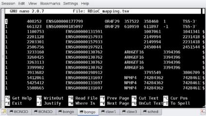
It should look like the screenshot above. Now change the cells ZFHX1B<TAB>ZEB2 to ZFHX1B;ZEB2 and additionally fix all the errors by changing the erroneous <TAB> to a ;. Once that’s done, we can re-run the script and find:
$ ./ff2bed_3.pl < RBioC_mapping.tsv > RBioC_mapping.bed
wrong # of values [6868]:
wrong # of values [6869]:
wrong # of values [6870]: *if non-existent uses Ensembl
The above shows the correct output - the comment lines are ignored & all lines process correctly except for the trailing 3 lines of the spreadsheet that contained 2 blank lines and a comment which we can ignore. The result looks like:
$ cols RBioC_mapping.bed
     0         1        2       3      4       5
#chrom  chrStart   chrEnd    name  score  strand
  chr1    408249   408252   clv_3    222       -
  chr1    661320   661323   clv_4    222       -
  chr1   1100750  1100753   clv_5    222       -
<etc>
which is what we want. (The name is a combination of a short string and the line number of the original SS data. Note that this will change if you re-run the data processing with different number of header lines in the original.
Also note that the input file had only a single peak value for the genomic position. A BED file requires a genomic range which requires that we fudge the data a bit - subtracting and adding 3 bases to produce such a range (indicated by the _3 in the script file name. We may use this ranging tweak again in the future.
bedtools, a suite of utilities for creating and working with the BED format is available on the BDUC cluster. The bedtools user manual is a very good description of how to work with the BED format and others like it.
So now we have a valid BED file to work on. Next is LiftOver.
7. LiftOver
LiftOver refers to the utility used to update the coordinates from one genomic assembly to another. In this case the data, were generated with the Human Build 17; the current version is 19. There are many differences between the two so this update is quite important.
The UCSC Genome Center provides a web page to do this as well as Linux and MacOSX binaries and the required chain files (the genome coordinate change files).
If you feed the web page the input file we’ve just created RBioC_mapping.bed, and select the Human builds converting from Build 17 to Build 19, you should generate a Results page which converts all the rows and and save it as a file named RBioC_mapping_19.bed
it should look like this:
$ cols RBioC_mapping_19.bed
   0        1        2       3    4  5
chr1   368386   368389   clv_3  222  -
chr1   621457   621460   clv_4  222  -
chr1  1060827  1060830   clv_5  222  -
<etc>
Now the input data is a state that can be manipulated with BioConductor.
8. R and BioConductor
R is a programming language that was developed for statistics and data analysis. BioConductor is a suite of specialized and optimized libraries and modules that are used within R to deal with genomic data.
R is mostly used interactively in a terminal. It can generate some very useful graphics but it is not a GUI program. In the following sections, I’ll demonstrate by providing mouseable commands that you can copy and paste into a terminal to generate the data along with me.
R can use a variety of internal structures to hold the data on which it operates. A common one is called a dataframe, a matrix of possibly different data types, much like a SS. If you’re interested in a very easy introduction to R, this page explains the basics and points to expanded introductions to R.
First, we need to read the previously created data file RBioC_mapping_19.bed into such a dataframe. We’ll use the read.table command to do this.
8.1. Starting R and loading needed Libraries
$ R  # that's right.  just 'R'

R version 2.10.1 (2009-12-14)
[Introductory text deleted]
>                           # the R prompt is '>'

# load the 'ChIPpeakAnno' library; the documentation is at:
# <http://www.bioconductor.org/packages/2.5/bioc/vignettes/ChIPpeakAnno/inst/doc/ChIPpeakAnno.pdf>

> library(ChIPpeakAnno)
Loading required package: biomaRt
Loading required package: multtest
Loading required package: Biobase
[many informational messages deleted]
Loading required package: limma
>
8.2. Getting your plain text data into R
While there are many ways to import and export data to and from R, I’ll use one of the simplest: read.table()
In the following line, replace /where/you/put/RBioC_mapping_19.bed with the real path name to the file. If you started R in the directory where the file is, you don’t need the leading path. ie just use RBioC_mapping_19.bed. The header=TRUE tells R that the 1st line is a header line and to map the names to the rest of the data.
# continuing from the same session as above...
> cl19 <- read.table(file="/where/you/put/RBioC_mapping_19.bed",header=TRUE)
# check it with str()
> str(cl19)
'data.frame':   6868 obs. of  6 variables:
 $ chrom   : Factor w/ 23 levels "chr1","chr10",..: 1 1 1 1 1 1 1 1 1 1 ...
 $ chrStart: int  368386 621457 1060827 2168963 2171136 2474591 3210000 3237265 3239953 3376742 ...
 $ chrEnd  : int  368389 621460 1060830 2168966 2171139 2474594 3210003 3237268 3239956 3376745 ...
 $ name    : Factor w/ 6868 levels "clv_10","clv_100",..: 1111 2222 3333 4444 5555 6536 6647 6758 1 112 ...
 $ score   : int  222 222 222 222 222 222 222 222 222 222 ...
 $ strand  : Factor w/ 2 levels "-","+": 2 1 1 2 2 1 2 2 2 2 ...
>
so cl19 is now a dataframe containing all the data from the file.
8.3. Convert the dataframe to RangedData
Now that data is in a dataframe named cl19 (could be called anything), the next line converts that dataframe into another specialized genomic data structure called RangedData.
# continuing from the same session as above...
> cl19rd <- BED2RangedData(cl19,header=FALSE)

# check it.  The next line prints out all of rows 1:4. The 23 'spaces' corresond to the 23 chromos
> cl19rd[1:4, ]
RangedData with 4 rows and 2 value columns across 23 spaces
            space             ranges |      strand     score
      <character>          <IRanges> | <character> <numeric>
clv_3           1 [ 621457,  621460] |          -1       222
clv_4           1 [1060827, 1060830] |          -1       222
clv_5           1 [2168963, 2168966] |           1       222
clv_6           1 [2171136, 2171139] |           1       222
8.4. Bringing networked databases into play
Now we use BioConductor’s useMart to load the Ensembl H.sapiens genome version GRCh37 (USCS’s Build 19 == Ensembl GRCh37)
# continuing from the same session as above...
mart<-useMart(biomart="ensembl",dataset="hsapiens_gene_ensembl")
Checking attributes ... ok
Checking filters ... ok

# incidentally, to use other datasets / marts
> othermart = useMart('ensembl')
> listDatasets(othermart)
                          dataset                                   description
1          oanatinus_gene_ensembl        Ornithorhynchus anatinus genes (OANA5)
2           tguttata_gene_ensembl       Taeniopygia guttata genes (taeGut3.2.4)
7           hsapiens_gene_ensembl                   Homo sapiens genes (GRCh37)
  ...
50          meugenii_gene_ensembl             Macropus eugenii genes (Meug_1.0)
51       cfamiliaris_gene_ensembl           Canis familiaris genes (CanFam_2.0)
<etc>
8.5. Extracting Genomic Annotations from the genome
If you wanted to search for all possible features, you could so at one go, using a featureType specification of ("TSS","miRNA", "Exon", "5utr", "3utr", "ExonPlusUtr") like this:
# continuing from the same session as above...
myFullAnnotation = getAnnotation(mart, featureType=c("TSS","miRNA", "Exon", "5utr", "3utr", "ExonPlusUtr"))

# takes several seconds
However, usually we’re interested in only a few features at the same time. If we want to use ONLY miRNA, then we search only for miRNA features by restricting the featureType:
# continuing from the same session as above...
myAnnotation = getAnnotation(mart, featureType=c("miRNA"))

# takes several seconds..
8.6. Map your data against the annotations
Now that the genomic annotations have been extracted into an R/BioConductor data structure called myAnnotation, we can compare our data (cl19rd in RangedData format) to it.
# continuing from the same session as above...
annotatedPeak = annotatePeakInBatch(cl19rd, AnnotationData = myAnnotation)

# takes several secs

# check the 1st 2 rows
> annotatedPeak[1:2,]
RangedData with 2 rows and 9 value columns across 23 spaces
                              space               ranges |        peak
                        <character>            <IRanges> | <character>
clv_100 ENSG00000238705           1 [28013340, 28013343] |     clv_100
clv_102 ENSG00000222787           1 [31297120, 31297123] |     clv_102
                             strand         feature start_position end_position
                        <character>     <character>      <numeric>    <numeric>
clv_100 ENSG00000238705           1 ENSG00000238705       26881033     26881084
clv_102 ENSG00000222787           1 ENSG00000222787       30357749     30357852
                        insideFeature distancetoFeature shortestDistance
                          <character>         <numeric>        <numeric>
clv_100 ENSG00000238705    downstream           1132307          1132256
clv_102 ENSG00000222787    downstream            939371           939268
                        fromOverlappingOrNearest
                                     <character>
clv_100 ENSG00000238705             NearestStart
clv_102 ENSG00000222787             NearestStart


# note that the RangedData format's are offset in elements so that you can
# get to the element you want directly
> annotatedPeak[1:3,0:3]
RangedData with 3 rows and 3 value columns across 23 spaces
                              space               ranges |        peak
                        <character>            <IRanges> | <character>
clv_101 ENSG00000222787           1 [31297120, 31297123] |     clv_101
clv_102 ENSG00000222787           1 [31863687, 31863690] |     clv_102
clv_103 ENSG00000221423           1 [32014775, 32014778] |     clv_103
                             strand         feature
                        <character>     <character>
clv_101 ENSG00000222787           1 ENSG00000222787
clv_102 ENSG00000222787           1 ENSG00000222787
clv_103 ENSG00000221423           1 ENSG00000221423
>
8.7. Intersects between your data and the genomic annotations
We can’t directly filter by maximum distance to feature, but we can do this post-query by restricting the output based on the distancetoFeature element (which can be selected by filtering on element [7]:
# continuing from the same session as above...

> annotatedPeak[1:3,7]
RangedData with 3 rows and 1 value column across 1 space
                             space             ranges | distancetoFeature
                       <character>          <IRanges> |         <numeric>
clv_10 ENSG00000130762           1 [3263113, 3263113] |           -107877
clv_11 ENSG00000130762           1 [3399902, 3399902] |             28912
clv_12 ENSG00000233304           1 [3913682, 3913682] |            -86991
>
8.8. Converting data from RangedData back to a dataframe
Most R functions use dataframes (or the simpler matrices) as their basic format, so we’re going to convert our RangedData back into a dataframe.
# continuing from the same session as above...

> mirna_df <- as.data.frame(annotatedPeak)
> mirna_df[1:3, ]
  space    start      end width                   names    peak strand
1     1 31297120 31297123     4 clv_101 ENSG00000222787 clv_101      1
2     1 31863687 31863690     4 clv_102 ENSG00000222787 clv_102      1
3     1 32014775 32014778     4 clv_103 ENSG00000221423 clv_103      1
          feature start_position end_position insideFeature distancetoFeature
1 ENSG00000222787       30357749     30357852    downstream            939371
2 ENSG00000222787       30357749     30357852    downstream           1505938
3 ENSG00000221423       33391895     33392000      upstream          -1377120
  shortestDistance fromOverlappingOrNearest
1           939268             NearestStart
2          1505835             NearestStart
3          1377117             NearestStart


# and finally look at the full names of the elements.
> names(mirna_df)
 [1] "space"                    "start"
 [3] "end"                      "width"
 [5] "names"                    "peak"
 [7] "strand"                   "feature"
 [9] "start_position"           "end_position"
[11] "insideFeature"            "distancetoFeature"
[13] "shortestDistance"         "fromOverlappingOrNearest"
>
8.9. Determining distances between our data and genomic features
Now we need to take only those rows from mirna_df in which the distancetoFeature (col [12]) is less than some value (10KB is what the PI wanted) and mark the closest "mirna" feature with col [12] (shortestDistance) [which gives direction] or col [13] (fromOverlappingOrNearest) which gives the absolute distance.
We could export this data and process it with Perl or (gaaacckkk) Excel as it’s not too big (~ same size as the input data) or we should be able to process it down to only those entries that have col [13] (fromOverlappingOrNearest) less than 10,000. Conveniently enough, there’s an R function called subset() that does just this, so we just append the conditions to extract the rows we want and presto!
# continuing from the same session as above...
> mirna_10k <- subset(mirna_df, mirna_df[,13] < 10000)

# now 'mirna_10k' has only those rows in which col [13] is < 10000

# check it on the 1st 3 rows
> mirna_10k[1:3,]
    space     start       end width                   names    peak strand
142     1 162319954 162319957     4 clv_335 ENSG00000207729 clv_335      1
286     1  67702373  67702376     4 clv_186 ENSG00000221733 clv_186     -1
290     1  68639888  68639891     4 clv_190 ENSG00000221203 clv_190     -1
            feature start_position end_position insideFeature distancetoFeature
142 ENSG00000207729      162312336    162312430    downstream              7618
286 ENSG00000221733       67705123     67705210    downstream              2837
290 ENSG00000221203       68649201     68649293    downstream              9405
    shortestDistance fromOverlappingOrNearest
142             7524             NearestStart
286             2747             NearestStart
290             9310             NearestStart

# see how many rows it has using str() which prints the dimensions of the data structure passed
> str(mirna_10k)
'data.frame':   114 obs. of  14 variables:
 <etc>
8.10. Exporting the data from R
There are only 114 rows in this subset, so we can write them out to a text file with:
# continuing from the same session as above...
write.table(mirna_10k, file="/where/to/write/mirna_10k.txt",quote = FALSE, sep = "\t",row.names = TRUE,col.names = TRUE)
>
The names column refer to the genomic feature identified as being the nearest miRNA within 10K bases of the peak. All that remains is to mail it to your supervisor with a suggested paper title.
9. Appendix
Until I modified scut to handle Excel files directly, I also described a way to do it via py_xls2csv. Since I wrote, I’ll retain it here.
$ py_xls2csv RBioC_Initial_Dataset.xls > RBioC_mapping.csv

# check the output ('cols' truncates the right edge of the field at the '--mw=xx' value)
$ cols --delim=',' --mw=10 <RBioC_mapping.csv
         0           1           2           3           4           5          6           7
Sheet = "S                                                                      -
----------                                                                      -
"Locations                                                                      -
"Chromosom   "TCF4 pea   "Closest    "Closest    "Gene sta   "Gene end   "Strand"   "Classifi
     "1.0"   "408252.0   "ENSG0000    "OR4F29"   "357522.0   "358460.0      "1.0"    "TSS-3'"
     "1.0"    "661323"   "ENSG0000    "OR4F29"    "610959"    "611897"     "-1.0"    "TSS-3'"
     "1.0"   "1100753"   "ENSG0000               "1007061"   "1041341"     "-1.0"   "5'-proxi
<etc>
py_xls2csv is fairly promiscuous in terms of defining variables as alphabetic strings and it sometimes quotes what are really numeric values, converting them to strings. Let’s clean up the file a bit with some judicious stream editing. You can use sed if you want; I like perl. The following lines do a global, case-insensitive, in-place string replacement, making a backup file (*.bak) as well.
$ perl -e 's/"//gi' -p -i.bak   RBioC_mapping.csv  # remove the quotes
# check it:
$ cols --delim=',' --mw=10 RBioC_mapping.csv       # quotes should be gone

$ perl -e 's/\.0//gi' -p -i.bak RBioC_mapping.csv  # remove the '.0' from some numeric
# check it:
$ cols --delim=',' --mw=10 RBioC_mapping.csv       # no more '.0's

$ perl -e 's/,/\t/gi' -p -i.bak RBioC_mapping.csv  # change the comma delimiter to a tab
# check it:
$ cols --mw=10 RBioC_mapping.csv        # delimiter is <TAB> now, but it shouldn't look different

$ tail -n+5 RBioC_mapping.csv > RBioC_mapping.tsv  # don't want those pesky header lines & rename
Now the file looks like this:
$ cols --mw=10 RBioC_mapping.tsv
         0           1           2           3           4           5        6           7
         1      408252   ENSG00000      OR4F29      357522      358460        1      TSS-3'
         1      661323   ENSG00000      OR4F29      610959      611897       -1      TSS-3'
         1     1100753   ENSG00000                 1007061     1041341       -1   5'-proxim
         1     2201128   ENSG00000                 2149994     2231418        1      TSS-3'
<etc>
(see?! everything is spiffy).
10. Latest Version
The latest version of this document will always be found here. The asciidoc source for this document is found here.