by Harry Mangalam <harry.mangalam@uci.edu> v0.2 - Jan 6th, 2016 :icons:
1. Preface
This tutorial is for researchers who are comfortable with Linux, but novices at cluster data analysis and especially dealing with BigData - data of various formats and faces that is too large to be handled by the techniques that you have may have used before - MS Word, Excel, pointy-clicky apps on your Mac and Windows. BigData is a tech term usually used these days in resumes to increase your salary demands and is often applied to very particular analytical techniques.
The preceding lecture and this extension / tutorial are NOT intended to be a definitive guide to specific BigData techniques - far from it. This document is meant to impart some very condensed real-life views on how data (Big and otherwise) lives, moves, can be convinced to jump thru hoops, some hints, and real life behavior of the same. It will emphatically not provide specific HOWTOs of current BigData techniques, but after reviewing it, you may be able to plan your approach in a more efficient way.
Hence the title being A Tourist’s Guide of BigData on Linux, not a HOWTO.
If you don’t know your way around a Linux bash shell nor how a compute cluster works, please review the previous Introduction to Linux essay/tutorial here. It reviews Linux, the bash shell, common commands & utilities, as well as the SGE scheduler. It’s pretty much a pre-requisite to this document.
2. Introduction
For those of you who are starting your graduate career and have spent most of your life with with MacOSX or Windows, the Linux commandline can be mystifying. The previous lecture and tutorial was meant to familiarize you with Linux on HPC, with only a very fast introduction to handling and analyzing large amounts of data.
You are the among the first few waves of the Data Generation - your lives and research guided by, and awash with, ever-increasing waves of data.
If you’re reading this, your research will almost certainly depend on large amounts of data, data that does not map well to MS Word, Excel, or other such pointy-clicky desktop apps. The de facto standard for large-scale data processing, especially in the research field, is the bash prompt, backed by a Linux compute cluster. It’s not pretty, but it works exceedingly well. In the end, I think you’ll find that it is worth the transition cost to use our cluster where most compute nodes each have 64 CPU cores, 1/2 TB of RAM and access to 100s of TB of disk space on a very fast parallel filesystem.
This is not a HOWTO on Analysis of BigData. That I’ll leave to others who have specific expertise. The aim of this document is to give you an idea of how data lives - how it is stored and unstored, what path it travels, and how much time it takes to transition from one state to another. I’ll touch briefly on some general approaches to analyzing data on the Linux OS, introducing some small-data approaches (which may be all you need) and then expanding them to much larger data.
3. Getting to BigData
BigData usually does not appear ready to go. It typically appears in large, unruly agglomerations of data in various states of undress. In order to feed it to your analyses, in most cases, you will need to:
-
download your data from somewhere on the internet, using wget, curl, ftp, etc.
-
extract the data you want using a combination of the grep family, cut, scut,
-
join disparate columns or parts of files together using scut, join, sqlite, pr, head, tail, etc.
-
clean and/or filter the data based on value, floor, ceiling, or comparison to other values
-
format and/or code it to make analysis easier or your data smaller.
-
section it into logical units or for parallel processing
-
stage it to optimal storage for max performance - to a parallel filesystem, to an SSD, to an in-memory filesystem or data structure.
-
Data Provenance is the history (or versioning) of your data, and the operations and analysis that have been done to it to that it’s repeatable. Think of this as your Data Lab Book.
|
|
Jupyter and Data Notebooks
Provenance is becoming VERY IMPORTANT due to many recent inabilities to replicate data analyses published in peer-reviewed journals. We provide Jupyter on HPC to assist in the creation of lab Data Notebooks that can be exchanged, edited, and re-run to enable others to replicate what you’ve done. These Data Notebooks are very sophisticated versions of your ~/.bash history which records the last 1000 or more commands you’ve performed. It can be reviewed with the command history. Try it. |
Here are some examples demonstrating the above points. These can and should be supplemented by your own google searches.
3.1. Regexes and the grep family
Also important in data-processing world is the idea of Regular Expressions (aka regexes), a formal description of patterns. There is a brief description in the previous tutorial and gobs more distributed over the Internet.
grep and grep-like utilities are possibly the most used utilities in the Unix/Linux world. These ugly but elegant utilities are used to search files for patterns of text called regular expressions and can select or omit a line based on the matching of the regex. The most popular of these is the basic grep and it, along with some of its bretheren are described well in Wikipedia. Another variant which behaves similarly but with one big difference is agrep, or approximate grep which can search for patterns with variable numbers of errors, such as might be expected in a file resulting from an optical scan or typo’s. Baeza-Yates and Navarro’s nrgrep is even faster, if not as flexible (or differently flexible), as agrep.
Regex searching is a key technique for filtering and cleaning data BEFORE you get to the stage of applying BigData techniques, a step that is often skipped by tutorials in BigData.
|
|
On HPC, qrsh to another node before doing any of the tutorial
Please use qrsh to log onto another node before you start these tutorials. Especially when multiple users do the same thing simultaneously it can cause a massive slowdown on the login nodes. Try the gpu queue: qrsh -q gpu # or qrsh -q test |
For example:
$ DDIR=bddir
$ mkdir $DDIR
$ cd $DDIR
$ wget http://moo.nac.uci.edu/~hjm/CyberT_C+E_DataSet
$ wc CyberT_C+E_DataSet
  600  9000 52673 CyberT_C+E_DataSet
# so the file has 600 lines.  If we wanted only the lines that had the
# identifier 'mur', followed by anything, we could extract it:

# (passed thru 'scut' (see below) to trim the extraneous cols.)
$ grep mur CyberT_C+E_DataSet | scut --c1='0 1 2 3 4'
b0085   murE    6.3.2.13        0.000193129     0.000204041
b0086   murF+mra        6.3.2.15        0.000154382     0.000168569
b0087   mraY+murX       2.7.8.13        1.41E-05        1.89E-05
b0088   murD    6.3.2.9 0.000117098     0.000113005
b0090   murG    2.4.1.- 0.000239323     0.000247582
b0091   murC    6.3.2.8 0.000245371     0.00024733
# if we wanted only the id's murD and murG:
$ grep mur[DG] CyberT_C+E_DataSet | scut --c1='0 1 2 3 4'
b0088   murD    6.3.2.9 0.000117098     0.000113005
b0090   murG    2.4.1.- 0.000239323     0.000247582


# also get a feeling for how scut can delete or rearrange the columns to your liking:
# what does this produce?

$ grep mur[DG] CyberT_C+E_DataSet | scut --c1='1 0 3 4'
Also see the first tutorial on slicing data.
3.2. cat
cat (short for concatenate) is one of the simplest Linux text utilities. It simply dumps the contents of the named file (or files) to STDOUT, normally the terminal screen. However, because it dumps the file(s) to STDOUT, it can also be used to concatenate multiple files into one.
$ cd $DDIR
$ wget http://moo.nac.uci.edu/~hjm/greens.txt
$ wget http://moo.nac.uci.edu/~hjm/blues.txt
$ cat greens.txt
turquoise
putting
sea
leafy
emerald
bottle

$ cat blues.txt
cerulean
sky
murky
democrat
delta

# now concatenate the files
$ cat greens.txt blues.txt >greensNblues.txt

# and dump the concatenated file
$ cat greensNblues.txt
turquoise
putting
sea
leafy
emerald
bottle
cerulean
sky
murky
democrat
delta
3.3. more & less
These critters are called pagers - utilities that allow you to page thru text files in the terminal window. less is a better more than more in my view, but it’s your terminal. These pagers allow you to queue up a series of files to view, can scroll sideways, allow search by regex, show progression thru a file, spawn editors, and many more things. Video example
$ less CyberT_C+E_DataSet
Below are some of the most common commands to be used either as options to less on the command-line or they can be entered from within less as well.
-
type h for help
-
type -N to number or UN-number the lines
-
type -S to fold or UN-fold the lines
-
type / to search for a pattern, n to search for the next hit of the same pattern,
-
type q for quit.
-
type 50p to move to 50% of the way thru the file
-
type > to go to the end of the file; < to go back to the top
-
type v to switch to editing the file; when you quit the editor, you’ll be dropped back into the pager. Note that the editor is determined by the settings of 2 environment variables: EDITOR and VISUAL which have to be set to your preferred editor. EDITOR refers to your preferred terminal editor; VISUAL refers to your preferred graphical editor
# if you want to use the vim editor, place the following in your ~/.bashrc.
export VISUAL=vim
export EDITOR=vim
3.4. head & tail
These two utilities perform similar functions - they allow you view the beginning (head) or end (tail) of a file. Both can be used to select contiguous ends of a file and pipe it to another file or pager. tail -f can also be used to view the end of a file continuously (as when you have a program continuously generating output to a file and you want to watch the progress). See this example for more on head and tail.
# NB: Often it's useful to trim the top 'K' lines from a file to remove
# a set of troublesome headers.  Use 'less -n +K' you want to do this, ie:

# what do you see when you execute:

$ head -5 CyberT_C+E_DataSet
# vs
$ tail -n +3 CyberT_C+E_DataSet | head -3
Note that the top 2 lines of the file were cut away; this technique can be piped to other applications to process as well.
3.5. cut & scut
These are columnar slicing utilities, which allow you to slice vertical columns of characters or fields out of a file, based on character offset or column delimiters. cut is on every Linux system and works very quickly, but is fairly primitive in its ability to select and separate data. scut is a Perl utility which trades some speed for much more flexibility, allowing you to select data not only by character column and single character delimiters, but also by data fields identified by any delimiter that a regex can define. It can also re-order columns (see example #above) and sync fields to those of another file, much like the join utility see below.
3.6. cols
cols is a very simple, but arguably useful utility that allows you to view the data of a file aligned according to fields. Especially in conjunction with less, it’s useful if you’re manipulating a file that has 10s of columns especially if those columns are of different widths. cols is explained fairly well here.
3.7. paste
paste can join 2 files side by side to provide a horizontal concatenation. ie:
$ cat file_1
aaa bbb ccc ddd
eee fff ggg hhh
iii jjj kkk lll

$ cat file_2
111 222 333
444 555 666
777 888 999

$ paste file_1 file2

aaa bbb ccc ddd         111 222 333
eee fff ggg hhh         444 555 666
iii jjj kkk lll         777 888 999
Note that paste inserted a TAB character between the 2 files, each of which used spaces between each field. See also this example.
3.8. join
join is a more powerful variant of paste that acts as a simple relational join based on common fields. join needs identical field values to finish the join. See that scut described above can also do this type of operation. For much more powerful relational operations, SQLite is a fully featured relational database that can do this reasonably easily (see below). A good example of join is here
4. The Line Eater
Use both of these in the form:
line-eater.py < some.text.file
Copy and paste into an editor, save them into an appropriate place, and don’t forget to chmod u+x line-eater.pl.
4.1. In Perl
#!/usr/bin/perl -w
# note the '-w' above; emits useful warnings
use strict;
while (<>) { # the line eater loop
  chomp; # clips the newline from the end of incoming lines
  print "Input Line = [$_]\n";  # prints the incoming line WITH a newline
  my $N = my @values = split(/ /);  # splits the incoming line on spaces
  # the values go into array '@values' and the number of them is in $N
  my $i = 0; # use $i as a counter
  while ($i < $N){  # while loop that counts up to 1 less than $N
    printf "> %s\n", $values[$i++];  # prints the individual values
                                     # and incr the $i
    sleep 1; # and waits 1s for you to see the result before looping
  }
}
4.2. In Python
#!/usr/bin/python
# NB: no 'strict' mode; python is fairly strict anyway
import sys,time # python has to 'import' specific libs to use them
token = ' ' # use 'token' to store the space; note no ';' endings
for line in sys.stdin: # the line-eater setup
        print "Input line:",  line   # print input line; does the output differ from Perl version?
        values = line.split(token);  # split on the token defined above
        for el in values:  # loop over each value in the line (now in 'values'
          print ">", el  # print out the word
        time.sleep(1) # what happens if you move this 1 tab to the right?
5. diff and related utils
Many of your analyses will require determining the differences between files. The diff family of utilities can identify differences on the level of line and even to the level of different characters.
If we stream-edit the CyberT_C+E_DataSet file to have a few substitutions..
# copy the file first:
cp CyberT_C+E_DataSet CyberT_C+E_DataSet.2

# change each instance of 'mur' with 'Mur'
perl -e 's/mur/Mur/gi' -p -i.bak CyberT_C+E_DataSet

# now find the differences, 1st with diff
diff CyberT_C+E_DataSet CyberT_C+E_DataSet.2 | less
# now with vimdiff
vimdiff CyberT_C+E_DataSet CyberT_C+E_DataSet.2
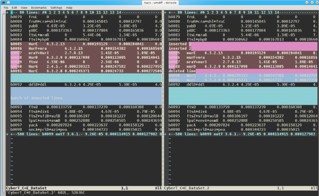 (see the interface difference?)
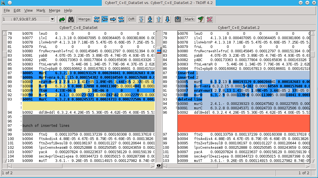
# if you have a graphical interface set up, you can use tkdiff
tkdiff CyberT_C+E_DataSet CyberT_C+E_DataSet.2
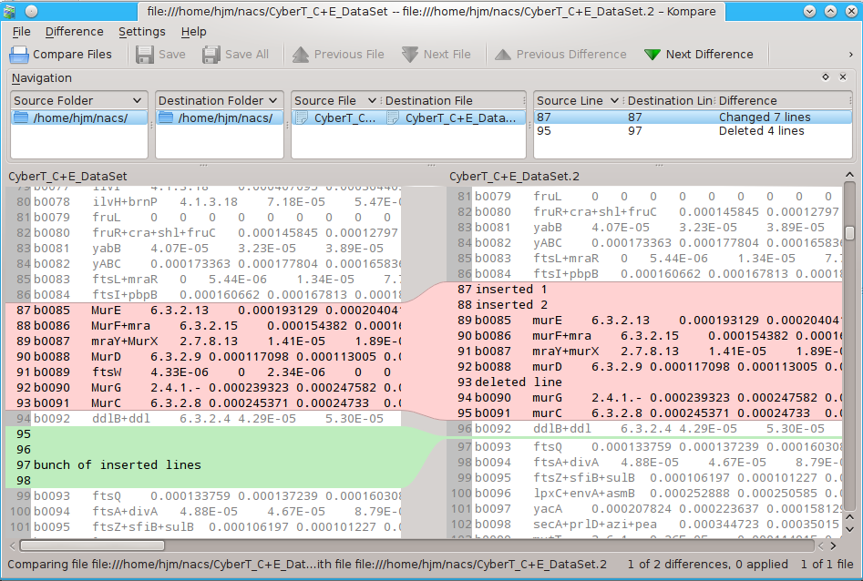
# and even kompare
kompare CyberT_C+E_DataSet CyberT_C+E_DataSet.2
5.1. Organizing your data
You can help your analysis by organizing your data more efficiently. See this link that shows one example of how to lay out ASCII data more efficiently.
The endpoint is that you should try to lay out your data to make it more convenient for the computer, not necessarily for you. This is a big step, involving experience and debugging, but it can result in orders of magnitude increases in speed of IO.
6. Binary format vs ASCII
Example?
7. Redirection and pipes
In the previous lecture & tutorial, I spent a lot of time describing the use of input-output (IO) redirection and especially its application to pipes and pipe-like devices. Please review that tutorial for some examples of redirection, pipes, why they’re very useful, how they work, with some examples].
8. The Data Flight Path
You might think of your analysis as a long airplane flight, say from LAX to Heathrow. One flight path is direct via the polar route. Another might be a series of short commuter flights that hops across the US to Florida and then up the east coast, eventually to Nova Scotia then to Gander, NFLD, and finally to Dublin, then to Edinburgh, then finally to Heathrow. The more times your plane has to land, the longer it will take. Data has the same characteristic, where landing is equivalent to being writ to disk. The more times your data has to be written to disk and read from it, the lower the whole analysis will take. Much of this doc describes techniques to either bypass (or mask) disk IO.
8.1. CPU registers
In order to be manipulated by the CPU, the binary data has to be in CPU registers - very small, very high speed storage locations inside the actual CPU die that are used to hold the data immediately being operated on: where the data comes from and where it’s supposed to go in RAM, the operations to be done, the state of the program, the state of the CPU, etc. These registers operate in sync with the CPU at the CPU clock speed, currently somewhere in the range of 3GHz, or one operation every 0.3 nanoseconds.
8.2. CPU cache
CPU cache is used to store the data coming into and out of the CPU registers and is often tiered into multiple levels, primary, secondary, tertiary, and even quaternary caches. These assist in staging data that the CPU is asking for or even that the CPU might ask (a speculative fetch) for based on the structure of the program it’s running and the compiler used.
The size of these caches has grown exponentially over the last few years as fabs can jam more transistors onto a die and caching algorithms have gotten better. In the Pentium era, a large primary cache used to be a few bytes. Now it’s 32KB, multi-thread accessible for the latest Haswell CPUs, with 256KB L2 cache, and 2-20MB L3 cache. These transistors are typically on the same silicon die as the CPU, mere microns away from the CPU, so the access times are typically VERY fast.
As the cache gets further away from the CPU registers, the time to access the data stored there gets slower as well. To use the data from a primary cache takes ~4 clock tics; to use data from the secondary cache takes ~11 tics, and so on down the line.
8.3. System RAM
System RAM, typically considered very fast, is actually very slow compared to the L1, L2, and L3 caches. It is further, both physically, as well as electronically, since it has to be mediated by a separate memory controller. To refresh data from main RAM to L1 cache takes on the order of 1000 clock tics (or a few hundred ns). So RAM is very slow compared to cache…
BUT! System memory access is a 1000 to 1M times faster than disk IO, in which the time to swing round a disk platter, position the head and initiate a new read is on the order of several to several 100 milliseconds, depending on the quality of disk, amount of external vibration, and anti-vibration features.
The preceding grafs have been to impress upon you that when your data is picked up off a disk, it should remain off disk as long as possible until you’re done analyzing it. Reading data off a disk, doing a small operation, and then writing it back to disk many times thru the course of an analysis is the among the worst offenses in data analysis. KEEP YOUR DATA IN FLIGHT.
8.4. Flash Memory / SSDs
In recent years, flash or non-volatile memory - which does not need power to keep the data intact - has gotten cheaper as well. You’re probably familiar with this type of memory in thumbdrives, removable memory for your phones and tablets, and especially SSDs. This memory is notable for HPC and BigData in that unlike spinning disks, the time to access a chunk of data is fairly fast - on the order of microseconds. The speed at which data can be read off in bulk is not much different than a spinning disk, but if your data is structured discontinuously or needs to be read and written in non-streaming mode (such as with many relational database operations), SSDs can provide a very high-performance boost because of the very low latency.
There is another issue with the memory currently being used in SSDs which is that because the transistors are so small, they can can actually wear out over time which is why SSDs typically have a huge oversupply of memory cells which are remapped into use as other cells die off. This problem is improving dramatically as both the logic controllers and the production of the chips improve.
8.5. RAM and the Linux Filecache
All modern OSs support the notion of a file cache - that is, if data has been read recently, it’s much more likely to be needed again. So instead of reading data into RAM, then clearing that RAM when it’s not needed, Linux keeps it around - stuffing it into the RAM that’s not needed for specific apps, their data, and other OS functions. This is why Linux almost never has very much free RAM - it’s almost all used for file pointers and the filecache (buffers & cached Mem, respectively in the top display below):
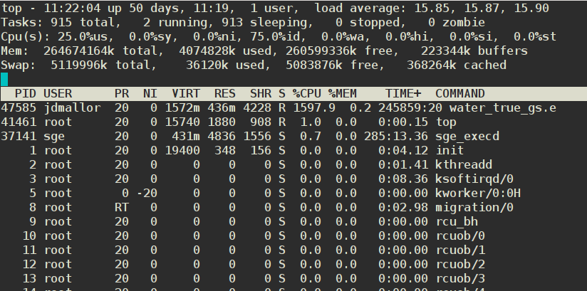
The OS only clears a chunk of filecache when the cached data has expired or when an app or the OS needs more. This is one reason why you should always prefer more RAM to a faster CPU when buying a new PC/Mac (which both use similar approaches to speeding up operations).
# 1st, create a 200MB file of random data (will take ~1 m)
$ dd if=/dev/urandom of=urandom.200M count=1000000 bs=200
1000000+0 records out
200000000 bytes (200 MB) copied, 45.9605 s, 4.4 MB/s

now copy it to another file (takes a couple of s)
$ cp urandom.200M urandom.200M.copy

# now, read it, immediately after clearing the filecache.
# Note that you will not be able to clear the filecache on HPC since it
requires root privs, but you can on your own Linux system via this command:

[root] # echo 3 > /proc/sys/vm/drop_caches
# see <http://goo.gl/3jD3Wa>

# ReadBinary.pl just reads binary data.

# wait for 1m to give the filecache a bit of time to clear.
$ time ReadBinary.pl  urandom.200M
Read 200000000 bytes

real    0m1.928s   <- took about 2 s


# repeated immediately afterwards from filecache.

$  time ReadBinary.pl  urandom.200M
Read 200000000 bytes

real    0m0.217s  < about 1/10th the time

# but if the identical file has another name..
$ time ./ReadBinary.pl  urandom.200M.copy
Read 200000000 bytes

real    0m1.922s < it isn't cached, so it'll take the original time.
|
|
Exploiting the FileCache
This can be exploited in real life by repeating reads on a file quickly if you need to re-read a file. Because of this caching behavior, it may be faster to do multiple simple operations on a file than 1 complicated one, depending on … many things. |
|
|
Streaming Data Input/Output (IO)
Streaming data Input/Output (IO) is the process (reading or writing) where the bytes are processed in a continuous stream. It usually refers to data on disk, where the time to change an IO point is quite significant (milliseconds). We often see this kind of data access in bioinformatics in which a large chunk of DNA needs to be read from end to end, or in other domains where large images or binary data need to be read into RAM for processing. The reverse of streaming IO is discontinuous IO, where a few bytes need to be read from one part of a file, processed, and then written to another or the same file. This type of data IO is often seen in relational database processing where a complex table join to answer a query results in very complicated data access patterns to locate all the data. Data on disk that can be streamed can be read much more efficiently than data that needs a lot of disk head movement. (see Inodes and Zotfiles immediately below). |
8.6. Inodes and Zotfiles
Each file that is stored on a block device (usual a disk) has to have some location metadata stored to allow the OS to find it and its contents; the directory structure associates the filename and this inode information. If you delete a file or dir, the file data is not lost formally, but the inode which is the pointer to that data is; in practice, the loss of the inode is effectively the loss of the data, unless you act very quickly to shut down the system and recover the data via extraordinary means (we will NOT do this for you if you accidentally delete a file on HPC).
Any file that is written to disk requires an inode structure entry, whether it’s 1 bit or 1TB. Usually there is a surplus of inodes on a filesystem, but if users start using lots of very small files, then the inodes can be used up quickly. This is known locally as the Zillions of Tiny file or ZOTfile problem.
Zotfiles are generally not a problem on your own system, but on a cluster, they are deadly - it takes approx the same time to process an inode for a file containing 1 byte as for one that contains 200GB. We have found users who had 40K files of <100 bytes in a dir, organizing/indexing those files by date, time, and a few variables.
DO NOT DO THIS; THIS IS .. UNWISE.
If you have lots of tiny amounts of data to write onto disk, write it to the SAME FILE, even if you’re writing to it from several processes. There is a mechanism called file-locking that allows multiple processes to write to the same file without data loss or even very much contention. We have documented this with examples.
For example, instead of opening a file with a clever name, writing a tiny amount of data into it, then closing it, you would open a file once, then write fields that index or describe the variables with the variables themselves in a single line (in the simplest case) to the same file until the run was done, then close the file. Those fields allow you to find the data in a post-process operation.
Or you could use a relational database engine like SQLite to write the data directly to a relational database as you go.
8.7. Disks and Filesystems
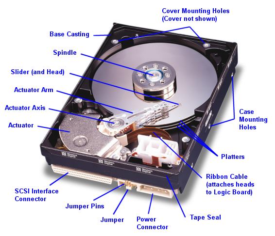
A hard disk is simply a few metal-coated disks spinning at 5K to 15K rpms with tiny magnetic heads moving back and forth on light arms driven by voice coils, much like the cones of a speaker. The magnetic heads either write data to the magnetic domains on the disks or read it back from those domains. However, because this involves accelerating and decelerating a physical object with great accuracy, as well as initiating the reads and writes at very precise places on the disk, it takes much longer to initiate an IO operation than with RAM or an SSD. Once the operation has begun, a disk can read or write data at about the same speed as an SSD (but typically much slower than RAM).
In order to increase either the speed or reliability of disks, they are often grouped together in RAIDs (Redundant Arrays of Inexpensive||Independent Disks) in which the disks can be used in parallel and/or with checksum parity to allow the failure of 1 or 2 disks in a RAID without losing data.
Such RAIDs are often used as the basis for a number of different filesystems, both local to a computer or via a network. In the latter case, the most popular protocol is the Network File System (NFS), which is reliable but complex and therefore somewhat slow. Individual RAIDs can also be agglomerated into larger networked arrays using various kinds of Distributed Filesystems (DFSs) in which a process (often running on a separate metadata server) tracks the requests for IO and tells the client where to send the actual bytes. Because the data can be read from or written to multiple arrays (each consisting of 10s of disks) simultaneously, the performance of such DFSs can be extremely high, 10s to 100s of times faster than individual disks. Examples of such DFSs are Gluster, BeeGFS/Fraunhofer, Lustre, OrangeFS, etc. On the UCI HPC cluster, we have 2 large BeeGFS parallel filesytems (/dfs1 & /dfs2) as well as a number of smaller ones.
9. Moving BigData
I’ve written an entire separate doc on this. Please read the Summary and also the section on avoiding data transfer.
9.1. rsync example
If you take nothing else from this class, learn how to use rsync. Here’s an example of how it works.
# create a directory tree and untar it
# first create a test dir, cd into it,
mkdir -p ~/rsync-test; cd ~/rsync-test;

# and then get the file and untar it in one line.
curl http://hpc.oit.uci.edu/biolinux/nco/nco-4.2.5.tar.gz | tar -xzf -
# or
curl http://moo.nac.uci.edu/~hjm/nco-4.2.5.tar.gz | tar -xzf -

# let's time how long it takes to rsync it to your laptop
# (only works with Macs, Linux, or Cygwin on windows)
# FROM YOUR LAPTOP
time rsync -av you@hpc.oit.uci.edu:~/rsync-test/nco-4.2.5 .

# note how much time it took.

# now let's edit 2 files in that tree to make them different, say
# 'INSTALL' and 'configure'.  Delete 2 lines in those files.
# (depending on what editor you use, it may make up a saved backup file named
# 'filename.bak' or 'filename~')

# now repeat the the rsync FROM YOUR LAPTOP
time rsync -av you@hpc.oit.uci.edu:~/rsync-test/nco-4.2.5 .

# how much time did it take that time?  Hopefully less.
rsync only copies the parts of the file that have changed, so in this case, it would have copied only the parts of those 2 files instead of the whole directory tree (as well as the complete backup files).
10. Data formats
There are a number of different data formats that compose data, Big or not.
10.1. Un/structured ASCII files
ASCII (also, but rarely, known as American Standard Code for Information Interchange) is text, typically what you see on your screen as alphanumeric characters altho the full ASCII set is considerably larger. For example, in bioinformatics, the protein and nucleic acid codes, as well as the confidence codes in FASTQ files are all ASCII characters. Most of this page is composed of ASCII characters. It is simple, human-readable, fairly compact, and easily manipulated by both naive and advanced programmers. It is the direct computer equivalent of how we think about data - characters representing alphabetic and numeric symbols. The main thing about ASCII is that it is character data - each character is encoded in 7-8bits (a byte). There is little correspondence between the symbol and its real value. ie. text symbol 7 is represented by ASCII value 55 decimal (base 0), 67 octal (base 8), 37 hexadecimal (base 16), and 00110111 in binary. The binary representation for the integer 7 is 111.
ASCII data is also notable for its use of tokens or delimiters. These are characters or strings that separate values in the data stream. These tokens are usually single characters like tabs, commas, or spaces, but can also be longer strings, such as __. These tokens not only separate values, but also take up space, one byte for each delimiter. For long lines of short data strings, this can eat up a lot of storage.
For many forms of data, and especially when that data gets very Big, ASCII data becomes less useful and takes longer to process. If you are a beginner in programming, you will probably spend the next several years programming with ASCII, regardless what anyone tells you. But there are other, more compact ways of encoding data.
10.2. Binary files
While all data on a computer is binary in one sense - the data is laid down in binary streams - binary format typically means that the data is laid down in streams of defined data types, segregated by format definitions in the program that does the reading. In this format, the bytes, integers, characters, floats, longs, and doubles of the internal representation of the data are written without intervening delimiter characters, like writing a sentence with no spaces.
163631823645618364912152ducksheepshark387ratthingpokemon
   \   \    \  \        \   \         \  \       \
%3d, %4d, %5d,%3d,%9.4f, %4s,  %10s,   %3d,  %8s, %7s  # read format
In the string of data above (translated into ASCII for readability), the string of numbers is broken into variables by the format string, an ugly, but very useful definition that for the above data string, looks like the read format line below it.
There is an additional efficiency with binary representation - data encoding. The 1st number 163 can be coded not in 3 bytes (1 byte each for the 1, the 6, and the 3), but in only 1 (which can hold 2^8 = 256 values). This is not so important when you only have 10 numbers to represent, but quite useful when you have a quadrillion numbers.
Similarly, a double-precision float (64bits = 8 bytes) can provide a precision of 15-17 significant digits while the ASCII representation of 15 digits takes 15 bytes.
For large data sets, the speed difference between using binary IO vs ASCII can be quite significant.
Another good explanation of the differences between ASCII/text and binary files is here.
10.2.1. Self-describing Data Formats
There are a variety of self-describing data formats. Self-describing can mean a lot of things from the extremely formalized such as the ASN.1 specification but it generally has a somewhat looser meaning - a format in which the description of the file’s contents - the metadata - is transmitted with the file, either as a header (as is the case with netCDF) or as inline tags and commentary (as is the case with Extensible Markup Language (XML)).
10.3. XML
XML is a variant of Standard Generalized Markup Language (SGML), the most popular variant of which is the ubiquitous Hypertext Markup Language (HTML) - by which a good part of the web is described. A markup language is a way of annotating a document in a way which is syntactically distinguishable from the text. Put another way, it is a way of interleaving metadata with the data to tell the markup processor what the data is. This makes it a good choice for small, heterogeneous data sets, or to describe the semantics of larger chunks of data, as used by the SDCubes format and the eXtensible Data Format (XDF).
However, because XML is an extremely verbose and repetitive data format (and therefore ~20x compressible), I’m not going to examine it in very much detail for this overview of BigData formats. Even if compressed on disk and decompressed while being read into memory, the computational overhead of filtering the data from the metadata makes it a poor choice for large amounts of data.
10.4. HDF5/netCDF4
The Hierarchical Data Format, which now includes HDF4, HDF5, and netCDF4 file formats is a very well-designed, self-describing data format for large arrays of numeric data and has even recently been adopted by some bioinformatics applications ( PacBio, BioHDF) dealing mostly with string data as well.
HDF files are supported by most widely used scientific software such as MATLAB (the default 7.3 version mat file is actually native HDF5) & Scilab, Mathematica, & SAS as well as general purpose programming languages such as C/C++, Fortran, R, Python, Perl, Java, etc. R and Python are notable in their support of the format.
HDF5/netCDF4 are particularly good for storing and reading multiple sets of multi-dimensional data, especially time-series data.
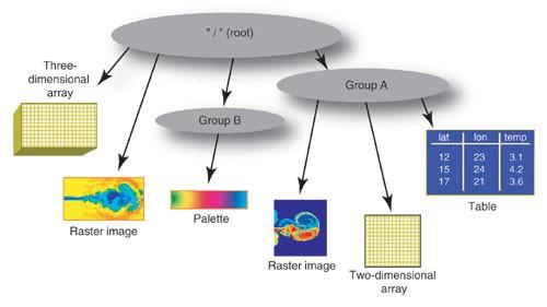
HDF5 has 3 main types of data storage:
-
Datasets, arrays of homogeneous types (ints, floats, of a particular precision)
-
Groups, collections of Datasets or other Groups, leading to the ability to store data in a hierarchical, directory-like structure, hence the name.
-
Attributes - Metadata about the Datasets, which can be attached to the data.
Advantages of the HDF5 format are that due to how the data is internally organized, access to complete sets of data is much faster than via relational databases. It is very much organized for streaming IO.
|
|
Promotional Note
Charlie Zender, in Earth System Science, is the author of nco, a popular set of utilities for manipulating and analyzing data in HDF5/netCDF format. This highly optimized set of utilities can stride thru such datasets at close-to-theoretical speeds and is a must-learn for anyone using this format. |
11. BigData file formats
|
|
The is a difference between HDFS and HDF5
Despite both being strongly associated with BigData and the acronymic similarity, HDFS (Hadoop File System) and HDF5 (Hierarchical Data Format) are quite different. HDFS is underlying special-purpose filesystem for Apache Hadoop. HDF5 is a file format for storing very large datasets. There is a very good good comparison between them, with the quotable summary line" Think of Hadoop as the single cup coffee maker and HDF5 as one form factor of coffee packs. |
There are a number of BigData file formats that are specialized for storing vast amounts of data, from Astronomy data to Satellite images to Stock Trading logs to Genomic data. Some examples are:
Some of these have been explicitly designed for a particular domain - the Flexible Image Transport System (FITS) format was designed for astronomical image data and isn’t used widely outside of that domain. However, files like the recently converging netCDF and HDF5 formats are general enough that they are now being used across a large number of domains, including bioinformatics, Earth System Science, Financial sectors, etc.
Due to the increasing size of Scientific data, we will be seeing more data supplied in this format, which does seem to be the next-gen version of ASCII data and already many commercial and OSS applications support it either in their base version or via plug-ins or libraries. Such apps include most of the usual suspects:
-
MATLAB (and MATLAB’s default .mat format IS apparently an HDF5 file with a funny header)
-
R, via the rhdf5 library
-
Python / NumPy / SciPy via h5py, (see here for example) Pytables, and ViTables.
-
Perl, via the Perl Data Language and the PDL::IO::HDF5 module.
-
Open Database Connectivity (ODBC) driver that allows an HDF5 file to be opened as a Database to allow import and export to just about any analytical system.
-
SAS - surprisingly, not so much
-
SPSS - surprisingly, not so much
Since the HDF5 format seems to be one of the better-supported BigData formats, we’ll take some time to examine it in more detail.
11.1. HDF5 format
I described how to read HDF5 files using R above, but this section will cover some other aspects of using them, especially how to view the contents in ways that are fairly easy to comprehend.
HDF5 is a hierarchical collection of hyperslabs - essentially a filesystem-like collection of multi-dimensional arrays, each composed of the same data type (like integers, floats, booleans, strings, etc). These array dimensions can be arbitarily extended in one dimension (usually time), and have a number of characteristics that make them attractive to very large sets of data.
And altho, you can access an HDF5 file sort of like a database (with the ODBC shim, noted above) and PyTables allows doing cross-array queries, it’s definitely NOT a relational data structure. Instead of being used to store relational data, it’s used to store very large amounts of (usually) numeric data that is meant to be consumed in entire arrays (or stripes thereof), analyzed or transformed, and then written back to another HDF5 array.
11.1.1. HDFView tutorial
For the HDF5-naive user, it is difficult to visualize what an HDF5 file looks like or how one is supposed to think about it. Herewith, a demo, one that requires the x2go client.
-
open the x2go client with the gnome terminal
-
If you haven’t already downloaded the test HDF5 file, please do it now.
# if from inside the cluster
wget http://nas-7-1/biolinux/bigdata/SVM_noaa_ops.h5

# if from outside the HPC cluster
wget  https://hpc.oit.uci.edu/biolinux/bigdata/SVM_noaa_ops.h5
-
Then load the HDF5 module
module load hdf5/1.8.13
hdfview.sh  #should launch the HDFView java app.
-
Now load the hdf5 file you just downloaded using the File interface
-
And click and double-click your way around them until you have an idea of what the variables and data represent.
-
Note the difference between single value variables, 1 & 2D arrays
-
Try to view the 2D arrays as images
-
Can you plot values?
11.1.2. Python & HDF5 tutorial
Python’s h5py library allows you to access all of the HDF5 API.
As an example of how to read a piece of an HDF5 file from Python, the following scriptlet can print out a 20x20 chunk of a specific Group variable. The problem is that you have to KNOW the the Group Variable name via HDFView or vitables.
# for this example, have to load some modules
module load openmpi-1.6.0/gcc-4.7.3
module load enthought_python/7.3.2

# to visualize the HDF5 internals and get the Variable names.

hdfview.sh  SVM_noaa_ops.h5 &  # works on HPC
# or
vitables    SVM_noaa_ops.h5 &  # may not be installed on HPC.
Following example adapted from here
#!/usr/bin/env python
'''Reads HDF5 file using h5py and prints part of the referenced array'''

import h5py    # HDF5 support

fileName = "SVM_noaa_ops.h5"
f = h5py.File(fileName,  "r")
for item in f.attrs.keys():
    print item + ":", f.attrs[item]

mr = f['/All_Data/VIIRS-M1-SDR_All/QF1_VIIRSMBANDSDR']

for i in range(20):
    print i,
    for j in range(20):
       print mr[i][j],
    print
f.close()
You can download the above code from here (and chmod +x read_hdf5.py) or start up ipython and copy each line in individually to see the result interactively. (in Python, indentation counts.)
There are sections of the previous tutorial that deal explicitly with reading data in the HDF5 format. See especially, the section about using HDF5 with R.
11.2. netCDF format
netCDF is another file format for storing complex scientific data. The netCDF factsheet gives a useful overview. In general, netCDF has a simpler structure and at this point, probably more tools available to manipulate the files (esp. nco). netCDF also allows faster extraction of small dataset from large datasets better than HDF5 (which is optimized for complete dataset IO).
Like HDF, there are a variety of netCDF versions, and with each increase in version number, the capabilities increase as well. netCDF is quite similar to HDF in both intent and implementation and the 2 formats are being harmonized into HDF5. A good, brief comparison between the 2 formats is available here. The upshot is that if you are starting a project and have to decide on a format, HDF5 is probably the better choice unless there is a particular advantage of netCDF that you wish to exploit.
However, because there are Exabytes of data in netCDF format, it will survive for decades, and especially if you use climate data and/or satellite data, you’ll probably have to deal with netCDF formats.
11.3. Relational Databases
If you have complex data that needs to be queried repeatedly to extract interdependent or complex relationships, then storing your data in a Relational Database format may be an optimal approach. Such data, stored in collections called Tables (rectangular arrays of predefined types such as ints, floats, character strings, timestamps, booleans, etc), can be queried for their relationships via Structured Query Language (SQL), a special-purpose language designed for this specific purpose.
SQL has a particular format and syntax that is fairly ugly but necessary to use. The previous link is from the SQLite site, but the advantage of SQL is that it is quite portable across Relational engines, allowing transitions from a relational Engine like SQLite to a fully networked Relational Database like MySQL or PostgreSQL.
11.4. SQL Engines & Servers
Structured Query Language is an extremely powerful language to extract information from data structures that have been designed to allow relational queries. That is, the data embedded in the tables have a defined relationship to each other.
There are overlaps in capabilities, but the difference between a relational engine like the lightweight SQLite relational engine and a networked database like MySQl is that the latter allows multiple users to read and write the database simultaneously from across the internet, while the former is designed mostly to provide very fast analytical capability for a single user on local data. For example, many of the small and medium size blogs, content management systems, and social networking sites on the internet use MySQL. Many client-side, single-user databases that support things such as music and photo databases and email systems use sqlite engines.
Here’s a simple example of using the Perl interface to SQLite to read a specified number of files from your laptop, create a few simple tables based on the data and metadata, and then allow you to query the resulting tables with a few simple queries.
# start at your HOME directory
$ cd

# get a small tarball to use as a target; this will pull down
# and unpack the source code
$ wget http://hpc.oit.uci.edu/biolinux/nco/nco-4.2.5.tar.gz
$ tar -xzvf nco-4.2.5.tar.gz

# now point the indexer at it

$ rm -f  filestats;    # to delete the previous database
$ recursive.filestats.db-sqlite.pl   --startdir nco-4.2.5 \
--maxfiles=1000
Start a [N]ew DB or [A]dd to the existing one? [A] N
setting PRAGMA default_synchronous = OFF
hit a key to start loading data, starting at nco-4.2.5 .
 ... goes to work ...
nco-4.2.5 only has 379 files, but you end up with a simple SQLite database that can be browsed with the sqlitebrowser GUI or via the commandline sqlite3 core application. The HPC cluster does not support the browser (yet, but let us know if you want it).
 $ sqlite3 filestats
SQLite version 3.6.20
Enter ".help" for instructions
Enter SQL statements terminated with a ";"
sqlite> .schema
CREATE TABLE content(
     fk_lo      integer REFERENCES location,
     filename   varchar(80),
     filetype   varchar(32),
     content    varchar(256)
);

  (dumps the schema as a series of CREATE TABLE listings.

# example single-table query:

sqlite> select loc.filename from location loc where loc.isize < 100;
.
TAG
.htaccess
VERSION

# only 3 files are < 100bytes

sqlite> select loc.filename from location loc where loc.isize < 300;
.
Makefile.am
ncap.in2
Makefile.am
ncap2.hh
TAG
man_srt.txt
.htaccess
README_Fedora.txt
VERSION

# so only those files above are less than 300 bytes.
See this SQL tutorial for more information on how to use SQL to extract more specialized information.
12. Timing and Optimization
If you’re going to be analyzing large amounts of Data, you’ll want your programs to run as fast as possible. How do you know that they’re running efficiently? You can time them relative to other approaches. You can profile the code using time and /usr/bin/time, oprofile, perf, or HPCToolkit among a long list of such tools.
12.1. time vs /usr/bin/time
time gives you the bare minimum timing info
# for the rest of this section:
module load tacg
INPUT=/data/apps/homer/4.7/data/genomes/hg19/chr1.fa
$ time tacg -n6 -S -o5 -s  < $INPUT  > out

real    0m10.599s
user    0m10.456s
sys     0m0.145s
/usr/bin/time give you more info, including the max memory the process used, and how the process used memory, including pagefaults.
$ /usr/bin/time ./tacg -n6 -S -o5 -s  < $INPUT > out

10.47user 0.14system 0:10.60elapsed 100%CPU (0avgtext+0avgdata 867984maxresident)k
0inputs+7856outputs (0major+33427minor)pagefaults 0swaps
'/usr/bin/time -v can give you even more info, including …
$ /usr/bin/time -v ./tacg -n6 -S -o5 -s  < $INPUT  > out
        Command being timed: "./tacg -n6 -S -o5 -s"
        User time (seconds): 10.46
        System time (seconds): 0.14
        Percent of CPU this job got: 100%
        Elapsed (wall clock) time (h:mm:ss or m:ss): 0:10.60
        Average shared text size (kbytes): 0
        Average unshared data size (kbytes): 0
        Average stack size (kbytes): 0
        Average total size (kbytes): 0
        Maximum resident set size (kbytes): 867268
        Average resident set size (kbytes): 0
        Major (requiring I/O) page faults: 0
        Minor (reclaiming a frame) page faults: 33147
        Voluntary context switches: 1
        Involuntary context switches: 1382
        Swaps: 0
        File system inputs: 0
        File system outputs: 7856
        Socket messages sent: 0
        Socket messages received: 0
        Signals delivered: 0
        Page size (bytes): 4096
        Exit status: 0
Oprofile is a fantastic, relatively simple mechanism for profiling your code.
Say you had a application called tacg that you wanted to improve. You would first profile it to see where (in which function) it was spending its time.
$ module load tacg
$ operf ./tacg -n6 -S -o5 -s  < $INPUT  > out
$ operf: Profiler started

$ opreport --exclude-dependent --demangle=smart --symbols ./tacg
Using /home/hjm/tacg/oprofile_data/samples/ for samples directory.
CPU: Intel Ivy Bridge microarchitecture, speed 2.501e+06 MHz (estimated)
Counted CPU_CLK_UNHALTED events (Clock cycles when not halted) with a unit mask
of 0x00 (No unit mask) count 100000
samples  %        symbol name
132803   43.1487  Cutting
86752    28.1864  GetSequence2
49743    16.1619  basic_getseq
9098      2.9560  Degen_Calc
7522      2.4440  fp_get_line
7377      2.3968  HorribleAccounting
6560      2.1314  abscompare
4287      1.3929  Degen_Cmp
2600      0.8448  main
704       0.2287  basic_read
212       0.0689  BitArray        <- should we optimize this function?
112       0.0364  PrintSitesFrags
3        9.7e-04  ReadEnz
3        9.7e-04  hash.constprop.2
2        6.5e-04  hash
1        3.2e-04  Read_NCBI_Codon_Data
1        3.2e-04  palindrome
You can see by the above listing that the program was spending most of its time in the Cutting function. If you had been thinking about optimizing the BitArray function, even if you improved it 10,000%, it could only improve the runtime by ~ 0.06%.
Beware premature optimization.
Using perf which is now preferred over oprofile
$ perf stat ./tacg -n6 -S -o5 -s  < $INPUT  > out

 Performance counter stats for './tacg -n6 -S -o5 -s':

      10691.816321 task-clock (msec)         #    0.842 CPUs utilized
              3403 context-switches          #    0.318 K/sec
               146 cpu-migrations            #    0.014 K/sec
            224184 page-faults               #    0.021 M/sec
       32043489221 cycles                    #    2.997 GHz
        9877730243 stalled-cycles-frontend   #   30.83% frontend cycles idle
   <not supported> stalled-cycles-backend
       36944531987 instructions              #    1.15  insns per cycle
                                             #    0.27  stalled cycles per insn
       10301160998 branches                  #  963.462 M/sec
         513338471 branch-misses             #    4.98% of all branches

      12.696812705 seconds time elapsed

# now use 'perf' to look inside what's happening in the tacg run

$ perf record -F 99 ./tacg -n6 -S -o5 -s  < $INPUT  > out

# the above command ran tacg and allowed perf to record the CPU
# metrics for that run.  To see them:

$ perf report
 40.01%  tacg  tacg               [.] Cutting
 23.95%  tacg  tacg               [.] GetSequence2
 14.03%  tacg  tacg               [.] basic_getseq
  4.75%  tacg  [kernel.kallsyms]  [k] 0xffffffff8104f45a
  2.62%  tacg  tacg               [.] HorribleAccounting
  2.53%  tacg  tacg               [.] fp_get_line
  2.32%  tacg  libc-2.19.so       [.] msort_with_tmp.part.0
  2.15%  tacg  tacg               [.] Degen_Calc
  2.06%  tacg  libc-2.19.so       [.] __ctype_b_loc
  1.58%  tacg  tacg               [.] __ctype_b_loc@plt
  1.31%  tacg  tacg               [.] abscompare
  0.74%  tacg  libc-2.19.so       [.] __memcpy_sse2
  0.65%  tacg  tacg               [.] Degen_Cmp
  0.65%  tacg  tacg               [.] main
  0.19%  tacg  libc-2.19.so       [.] vfprintf
  0.09%  tacg  tacg               [.] DD_Mem_Check
  0.09%  tacg  tacg               [.] basic_read
  0.09%  tacg  libc-2.19.so       [.] __fprintf_chk
  0.09%  tacg  libc-2.19.so       [.] strlen
  0.09%  tacg  libc-2.19.so       [.] _IO_file_xsputn@@GLIBC_2.2.5

# you can punch down to examine the 'hotspots' in each function as well.
13. Compression
There are 2 types of compression - lossy and lossless. Lossless compression indicates that a compression/decompression cycle will exactly reconstruct the data. Lossy compression means that such a cycle results in loss of original data fidelity.
Typically for most things you want lossless compression, but for some things, lossy compression is OK. The market has decided that compressing music to mp3 format is fine for consumer usage. Similarly, compressing images with jpeg compression is fine for most consumer use cases. Both these compression algorithms use the tendency for distributions to be smooth if sampled frequently enough and to be able to approximate the original distribution of data well enough when reconstructing the waveform or colorspace. The well enough part of this is why some ppl don’t like mp3 sound and images that have been jpeg-compressed will appear oddly pixellated at high magnification, especially in low-contrast areas.
The amount of compression you can expect is also variable. Compression typically works by looking for repetition in nearby blocks of data. Randomness is the opposite of repetition, so ..
13.1. Random data
# You can re-use the random data that we generated above, or generate it again.

$ dd if=/dev/urandom of=urandom.200M count=1000000 bs=200
  ====

$ ls -l urandom.200M
-rw-r--r--  1 root     root   200000000 Nov 23 13:27 urandom.200M

$ time gzip urandom.200M
real    0m10.938s
  ====
ls -l urandom.200M.gz
-rw-r--r-- 1 hmangala staff 200031927 Nov 23 13:27 urandom.200M.gz
# So compressing nearly random data actually results in INCREASING
# the file size.

# incidentally, lets test pigz, the parallel gzip:

$ time pigz -p8 urandom.200M.copy

real    0m2.952s

# so using 8 cores, the time taken to compress the file decreases about 3.7X,
# not perfect, but not bad if you have spare cores.
13.2. Repetitive Data
However, compressing pure repetitive data from the /dev/zero device:
# make the zero-filled file:
$ time dd if=/dev/zero of=zeros.1G count=1000000 bs=1000

$ ls -l zeros.1G
-rw-r--r-- 1 hjm hjm 1000000000 Nov 14 11:31 zeros.1G
  ====
$ time gzip zeros.1G
real    0m7.100s
  ====
 $ ls -l zeros.1G.gz
-rw-r--r-- 1 hjm hjm 970510 Nov 14 11:32 zeros.1G.gz
So compressing 1GB of zeros took considerably less time and resulted in a compression ration of ~1000X. Actually, it should be smaller than that, since it’s all zeros.
And in fact, bzip2 does a much better job:
$ time bzip2 zeros.1G
real    0m10.106s
  ====
$ ls -l zeros.1G.bz2
-rw-r--r-- 1 hjm hjm 722 Nov 14 11:32 zeros.1G.bz2
or about 1.3 Million fold compression, about the same as Electronic Dance Music.
For comparison sake, a typical JPEG image easily achieves a compression ratio of about 5-15 X without much visual loss of accuracy, but you can choose what compression ratio to specify.
The amount of time you should dedicate to compression/decompression should be proportional to the amount of compression possible.
ie; Don’t try to compress an mp3 of white noise.
14. Moving BigData
I’ve written an entire document How to transfer large amounts of data via network about moving bytes across networks, so I’ll keep this short.
As much as possible, Don’t move the data. Find a place for it to live and work on it from there. Hopefully, it’s in compressed format so reads are more efficient.
Everyone should know how to use rsync, if possible the simple commandline form:
rsync -av /this/dir/   you@yourserver:/that/DIR
#                  ^
# note that trailing '/'s matter.
# above cmd will sync the CONTENTS of '/this/dir' to '/that/DIR'
# generally what you want.

rsync -av /this/dir   you@yourserver:/that/DIR
#                  ^
# will sync '/this/dir' INTO '/that/DIR', so the contents of '/that/DIR' will
# INCLUDE '/this/dir' after the rsync.
If you have lots of huge files in a few dirs, and it’s not an incremental move (the files don’t already exist in some form on one of the 2 sides), then use bbcp, which excels at moving big streams of data very quickly using multiple TCP streams. Note that rsync almost always will encrypt the data using the ssh protocol, whereas bbcp will not. This may be an issue if you copy data outside the cluster.
15. Processing BigData: Embarrassingly Parallel solutions
One key to processing BigData efficiently is that you HAVE to exploit parallelism (parallel = //). From filesystems to archiving and de-archiving files to moving data to the actual processing - leveraging //ism is the key to doing it faster.
The easiest to exploit is what’s called embarrassingly // (EP) operations - those which are independent of workflow, other data and order-of-operation. This analyses can be done by subsetting data and farming it out in bulk to multiple processes with wrappers like:
15.1. Gnu Parallel & clusterfork
Gnu Parallel and clusterfork are wrappers that allow you to write a single script or program and then directly shove it to as many other CPUs or nodes as are available to you, bypassing the need for a scheduler (and therefore are appropriate only for your own set of machines, not a cluster). Therefore while we have installed Gnu Parallel, we don’t recommend it for users due to it bypassing the SGE scheduler which keeps track of and allocates resources for the whole cluster.
Gnu Parallel is quite popular as a tool for users to increase the usage of their own machines, to the extent that there are extensive tutorials and even videos about its use.
clusterfork is like a parallel ssh that sends out commands to multiple machines, collects the results and identifies which results are identical. It’s being used heavily on HPC as an administrative tool, but it is not as well-developed as GNU Parallel for general purpose use.
15.2. SGE Array Jobs
To remind you of what a qsub script is and how it’s structured, please review the section on qsub scripts in the previous tutorial, especially the longer annotated one.
The Sun Grid Engine scheduler used on HPC has specific support for what is called an array job (aka job-array as well), a batch job that allows you to generate a sequence of numbers in a special variable called the SGE_TASK_ID and then use that variable to direct the execution of multiple (even thousands) of serial jobs simultaneously.
The advantage to doing it this way is that you don’t have to generate the 10s or 100s or even 1000s of shell scripts to run these jobs. The single, generally pretty simple qsub script will take care of all that for you, plus it’s MUCH easier on the head node which has to keep track of all the jobs, plus you can manipulate all the jobs simultaneously via the SGE q commands (qstat, qdel, qmod).
The special variable SGE_TASK_ID is specified with a single line in the SGE directives as shown below in the annotated qsub script.
#!/bin/bash

# specify the Q to run in, in the following case, any of the free Qs
#$ -q free*

# the qstat job name
#$ -N jobarray

# use the real bash shell
#$ -S /bin/bash

# execute the job out of the current dir and direct the error
# (.e) and output (.o) to the same directory ...
#$ -cwd

# ... Except, in this case, merge the output (.o) and error (.e) into one file
# If you're submitting LOTS of jobs, this halves the filecount and also allows
# you to see what error came at what point in the job.
# Recommended unless there's good reason NOT to use it.
#$ -j y

#!! NB: that the .e and .o files noted above are the STDERR and STDOUT,
#!! not necessarily the programmatic output that you might be expecting.
#!! That output may well be sent to other files, depending on how the app was
#!! written.

# !!!!!!!!!!!!!!!!!!!!!!!!!!!!!!!!!!!!!!!!!!!!!!!!!!!!!!!!!!!!!!!!!!!!!!!
# If you're using array jobs !!ABSOLUTELY DO NOT USE email notification!!
# !!!!!!!!!!!!!!!!!!!!!!!!!!!!!!!!!!!!!!!!!!!!!!!!!!!!!!!!!!!!!!!!!!!!!!!
# ie make sure the lines like the following are commented out like these are.

# mail me (hmangala@uci.edu)
## #$ -M hmangala@uci.edu
# when the job (b)egins, (e)nds, (a)borts,
## #$ -m bea

# Here is the array-job iteration notification and specification.
# This line will notify SGE that this job is an array-job and cause the
# internal variable $SGE_TASK_ID to run from 1 to 100
# NB: for reasons unclear, $SGE_TASK_ID will not run from 0-99, so
# if you require that series, you'll have to do some bashmath to generate it.
#$ -t 1-100

###### END SGE PARAMETERS  ######

###### BEGIN BASH SCRIPT   ######
# gumbo is a fake application which exists only in this example and in
# Louisiana cuisine
module load gumbo/3.43

# Assume INPUT_DIR has all the input files for this run, named from
# arctic_1_params to arctic_100_params
INPUT_DIR=/data/users/hmangala/gumbo/param_space

# Assume OUTPUT_DIR will receive all the respective output files
# arctic_1_result to arctic_100_result

OUTPUT_DIR=/data/users/hmangala/gumbo/param_space/results

# here's the commandline that actually runs the analysis
gumbo --input=${INPUT_DIR}/arctic_${SGE_TASK_ID}_params \
--globalsquish=4.62 \
--voidoid_capacity="dark" \
--opacity=3.992 \
--furting=128
--output=${OUTPUT_DIR}/arctic_${SGE_TASK_ID}_result

###### END BASH SCRIPT   ######
If the above qsub script was submitted, it would have run the 100 jobs in parallel, generating all the output files nearly simultaneously.
This shows how on a cluster, you can exploit the scheduler (SGE in our case) to submit hundreds or thousands of jobs to distribute the analysis to otherwise idle cores (and there are generally lots of idle cores). Note that this approach requires a shared file system so that all the nodes have access to the same file space.
This implies that the analysis (or at least the part that you’re //izing) is EP. And many analyses are - in simulations, you can often sample parameter space in parallel; in bioinformatics, you can usually search sequences in //;
15.3. Hadoop and MapReduce
This is a combined technique; it is often referred to by either terms but Hadoop is the underlying storage or filesystem that feeds the analytical technique of MapReduce. Rather than being a general approach to BigData, this is actually a very specific technique that falls into the EP area and is optimized for fairly specific, usually fairly simple operations. It is actually a very specific example of the much more general approach of cluster computing that we do
Wikipedia has this good explanation of the process.
-
Map step: Each worker node applies the map() function to the local data, and writes the output to a temporary storage. A master node orchestrates that for redundant copies of input data, only one is processed.
-
Shuffle step: Worker nodes redistribute data based on the output keys (produced by the map() function), such that all data belonging to one key is located on the same worker node.
-
Reduce step: Worker nodes now process each group of output data, per key, in parallel.
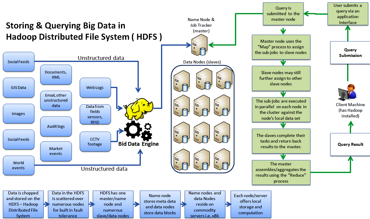
However, for those operations, it can be VERY fast and especially VERY scalable. One thing that argues against the use of Hadoop is that it is not a POSIX filesystem. It has many of the characteristics of a POSIX FS, but not all, especially a number related to permissions. It also is optimized for very large files and gains some robustness by data replication, typically 3-fold. If you use a general-purpose parallel filesystem such as HPC’s BeeGFS, you gain most of the speed of Hadoop with less complexity. You also have the flexibility to use non-MapReduce analyses.
An improvement on the MapReduce approach is a related technology Spark, which provides a more sophisticated in-memory query mechanism instead of the simpler 2-step system in MapReduce. As mentioned above, anytime you can maintain data in-RAM, your speed increases by at least 1000X. Spark also provides APIs in Python and SCALA as well as Java.