1. Introduction
This is an introduction to Linux specifically written for the HPC Compute Cluster at UCI. Replace the UCI-specific names and addresses and it should work reasonably well at your institution. Feel free to steal the ASCIDOC src and modify it for your own use.
This is presented as a continuous document rather than slides since you’re going to be going thru it serially and it’s often easier to find things and move around with an HTML doc. About half of this tutorial is about Linux basics and bash commands. The remainder covers a little Perl and more R.
|
|
Mouseable commands
The commands presented in the lightly shaded boxes are meant to be moused into the bash shell to be executed verbatim. If they don’t work, it’s most likely that you’ve skipped a bit and/or haven’t cd’ed to the right place. Try to figure out why the error occurred, but don’t spend more than a couple minutes on it. Wave one of us down to help. |
2. Logging In
3. On Campus vs Off Campus
To decrease the number of malware attacks, HPC is blocked from connection off-campus (including from University Hills). If you are off-campus, you’ll have to connect via an ssh connection to an on-campus machine 1st or via UCI’s Virtual Private Network connection. The VPN clients are freely available from OIT via the Software VPN tab on the link above.
3.1. ssh
We have to connect to HPC with ssh or some version of it so let’s try the basic ssh. If you’re using a Mac laptop, open the Terminal App (or the better, free iTerm (and type:
ssh -Y YourUCINETID@hpc.oit.uci.edu
# enter YourUCINETID password in response to the prompt.
3.1.1. via Putty
If you’re using Windows and the excellent, and free putty, (you’ll need only putty.exe), type UCINETID@hpc.oit.uci.edu into the Host Name (or IP Address) pane, and then your UCINETID password wen prompted. Once you connect, you can save the configuration and click the saved configuration the next time.
3.1.2. via Cygwin
If you are using the equally free and excellent Cygwin Linux emulator for Windows, you can use its terminal application to log in with the included ssh application.
3.1.3. via MobaXterm
mobaxterm is a commercial take on some of Cygwin’s components, with some of the rough edges sanded down, and some extra features added in. I’d recommend trying the free version. It’s gotten good reviews, but note that it is a commercial product and it will keep bugging you to upgrade to the $$ version. Up to you.
3.1.4. Passwordless ssh (plssh)
If you follow the instructions at this link, you’ll be able to log in to HPC without typing a password. That is extremely convenient and is actually more secure than typing the password each time (someone shoulder-surfing can peek at your fingers). However, since the private key resides on your laptop or desktop, anyone who has access to your computer when you’re logged in has access to your HPC account (and any other machines for which you’ve added a plssh login).
If you use plssh, there is another level of security that you can use, called ssh agent which protects your keys against this kind of attack. Essentially, it is a password for your ssh keys, unlocking them for the life of your shell session, then locking them again so that if someone steals your laptop, your ssh keys can’t be used to attack another system. Layers and layers….
4. Your terminal sessions
You will be spending a lot of time in a terminal session and sometimes the terminal just screws up. If so, you can try typing clear or reset which should reset it.
# reset your terminal
clear
#      or
reset
#      or
^r   # Ctrl +'r'
If all else fails, log out and then back in. Or kill the current screen/byobu session and re-create it with
^D  # (Ctrl + 'd')
# or
exit
# or
logout

# from within 'screen' or 'byobu'
^ak   # (Ctrl + 'a', then  'k'); this force-kills the current window

# then recreate it
^ac   # (Ctrl + 'a', then  'c'); this re-creates the missing session
4.1. screen/byobu
You will often find yourself wanting multiple terminals to hpc. You can usually open multiple tabs on your terminal emulator but you can also use the byobu app to multiplex your terminal inside of one terminal window. Byobu is a thin wrapper on GNU Screen which does all the hard work. Good help page on byobu here.
The added advantage of using byobu is that the terminal sessions that you open will stay active after you detach from them (usually by hitting F6). This allows you to maintain sessions across logins, such as when you have to sleep your laptop to go home. When you start byobu again at HPC, your sessions will be exactly as you left them.
|
|
A byobu shell in not quite the same as using a direct terminal connection
Because byobu invokes some deep magic to set up the multiple screens, X11 graphics invoked from a byobu-mediated window will sometimes not work, depending on how many levels of shell you’re in. Similarly, byobu traps mouse actions so things that might work in a direct connection (mouse control of mc) will not work in a byobu shell. Also some line characters will not format properly. Always tradeoffs… |
Hints:
-
tmux is a newer and more updated screen work-alike.
-
a good screen cheat sheet is here.
-
if you want a nice printable version
4.2. x2go
x2go is a client application that allows your laptop or desktop to display the X11 graphics that Linux/Unix OSs use. In addition to visualizing the graphics, it also acts as a data stream compressor that makes the display much more responsive than it would without using it. Especially if you’re trying to use a graphics program on the HPC cluster from off-campus, you really need the x2go client.
4.2.1. Macintosh installation
The Mac install requires a specific set of versions and steps.
-
Recent OSX releases do not include X11 compatibility software, now called XQuartz (still free). If you have not done so already, please download and install the latest version (2.7.7 at this writing). The x2go software will not work without it. After you install it and start it, please configure it to these specifications:
-
The XQuartz must be configured to "Allow connections from network clients" (tip from David Wang).
-
After installation of XQuartz, the user has to log out of the current Mac session and log back in again.
-
XQuartz must be running before starting x2go.
-
You may have to change your Mac’s Security Preferences to allow remote sessions.
-
If you’re running an additional local or personal firewall, you may have to specifically allow x2go to work.
-
-
Please install the Mac OSX client from here. The latest version (4.0.3.1, as of this writing) works on the Mavericks MacOSX release.
If your x2go DOESN’T work, please check the following:
-
Open Terminal.app, run ssh -X -Y yourname@hpc.oit.uci.edu, and , once you logged in to HPC, type xload and see if it opens a window showing the login node name.
-
If it says "Error: Can’t open display: ", please download the latest version of XQuartz and reinstall it (even if you already have latest version installed). You will need to logout then log back in after the installation. Please make sure to uncheck "Reopen windows when logging back in" option when logging out. You can download XQuartz from here: http://xquartz.macosforge.org/
-
Make sure you have the latest version of x2go
-
Reset all the x2go settings on your Mac by removing the .x2go and .x2goclient dirs in your home directory with the command:+ rm -rf ~/.x2go \~/.x2goclient
-
If you have any firewall on, please make sure x2go is in the whitelist. (OS X’s built-in firewall is off by default).
See below for x2go configuration to connect to HPC.
(x2go version compatibility changes fairly frequently, so if the above versions don’t work, please send me email.)
4.2.2. Windows installation
The Windows installation is straightforward and follows the instructions listed here.
4.2.3. x2go configuration for HPC
Configure your x2go client to connect to HPC using this screenshot as a guide, replacing hmangala with your UCINETID.
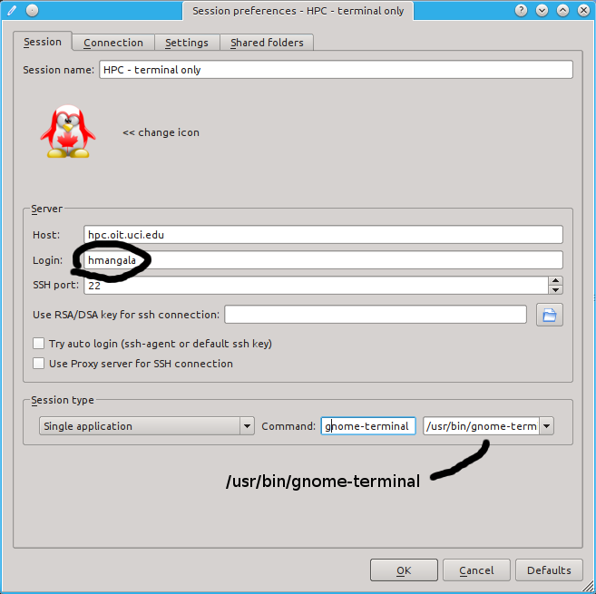
ONLY if you have added your public ssh key to your HPC account as described here, you can CHECK the option:
[x] Try auto login (ssh-agent or default ssh key)
If you haven’t set up passwordless ssh, UNCHECK it and use your UCINETID password in the password challenge box that comes up when you click OK.
Change the Session type to that shown: Single Application with the terminal application gnome-terminal (/usr/bin/gnome-terminal). When you configure it like this, only a terminal will pop up and then you can use it as a terminal as well as to launch graphical applications from it.
If you still cannot get your x2go client to work as expected, this page has a longer, more detailed explanation.
You can start other specific applications (such as SAS or SPSS) by entering the startup commands in the newly opened terminal. ie: module load rstudio; rstudio
5. Make your prompt useful
The bash shell prompt is, as almost everything in Linux, endlessly customizable. At the very least, it should tell you what time it is, what host you’ve logged into, and which dir you’re in.
Just paste this into a shell window. (This should work via highlighting the text and using the usual Copy/Paste commands, but depending on which platform you’re using, it may take some effort to get the right key combinations.
PS1="\n\t \u@\h:\w\n\! \$ "

# if you want to get really fancy, you can try this for a multicolored
# one that also shows the load on the system:

PS1="\n\[\033[01;34m\]\d \t \[\033[00;33m\][\$(cat /proc/loadavg | cut -f1,2,3 -d' ')] \
  \[\033[01;32m\]\u@\[\033[01;31m\]\h:\[\033[01;35m\]\w\n\! \$ \[\033[00m\]"

# that one will show up OK on most background, but on some light colored
# ones might wash out.
There is a reason for this. When you report a bug or problem to us, it’s helpful to know when you submitted the command, how busy the system was, and where you were when you submitted it. Including the prompt lets us know this info (most of the time).
OK - let’s do something.
|
|
Assumptions
I’m assuming that you’re logged into a bash shell on a Linux system with most of the usual Linux utilities installed. You should create a directory for this exercise - name it anything you want, but I’ll refer to it as $DD for DataDir. You can as well by assigning the real name to the shell variable DDIR: export DD=/the/name/you/gave/it cd $DD # go into it so we don't mess up any other dirs |
6. Simple Commands
6.1. Commandline Editing
Remember:
-
↑ and ↓ arrows scroll thru your bash history
-
^R will reverse-search thru your bash history (really useful)
-
← and → cursor thru the current command
-
the Home, End, Insert, and Delete keys should work as expected.
-
PgUp and PgDn often don’t work in the shell; if not, try Shift+PgUp/Down.
-
as you get comfortable with the commandline, some ppl like to keep their fingers on the keypad, so
-
^ means Ctrl
-
^a = Home (start of line)
-
^e = End (end of line)
-
^u = deletes from cursor to the start
-
^k = deletes from cursor to end of line
-
^w = deletes left from cursor one word ←
-
Alt+d = deletes right from cursor one word →
-
the ^ key amplifies some editing functions in the bash shell, so that ^ ← and ^ → will move the cursor by a word instead of by a char.
-
as noted above, sometimes your terminal keymaps are set wrong. Entering
setxkbmap -model evdev -layout us
into the terminal will often fix the mappings.
Also, while the following are not editing commands, you might accidentally type them when you’re editing:
-
^s = means stop output from scolling to the terminal (locks the output)
-
^q = means restart output scolling to the terminal (unlocks the output)
6.2. Aliases
At exactly the 27th time you’ve typed: ls -lht | head -22 to see the newest files in the current dir, you’ll wonder "Isn’t there a better way of doing this?". Yes. Aliases.
As the name implies, these are substitutions that shorten common longer commands.
alias nu='ls -lht | head -22'
now when you want to see the newest files, just type nu. You could name it new, but there’s a mail program called that.
What would the following aliases do?
alias toolbar-reset="killall plasmashell && kstart plasmashell 2>/dev/null"
alias bs1="ssh -Y hmangala@bs1"
alias obstat="ssh root@obelix '/usr/StorMan/arcconf GETSTATUS 1'"
alias sdn="sudo shutdown -Ph -g0 now"  # be careful with this one on your linux box
And when you want to make it permanent? Append it to your /.bashrc or to a separate file that is sourced from your /.bashrc. The following line will append the nu alias to your ~/.bashrc and therefore make it available every time you log in. Note the single and double quotes.
echo "alias nu='ls -lht | head -22'" >> ~/.bashrc
6.3. Copy and Paste
The copy and paste functions are different on different platforms (and even in different applications) but they have some commonalities. When you’re working in a terminal, generally the native platform’s copy & paste functions work as expected. That is, in an editing context, after you’ve hilited a text selection' Cntl+C copies and Cntl+V pastes. However, in the shell context, Cntl+C can kill the program that’s running, so be careful.
Linux promo: In the XWindow system, merely hiliting a selection automatically copies it into the X selection buffer and a middle click pastes it. All platforms have available clipboard managers to keep track of multiple buffer copies; if you don’t have one, you might want to install one.
6.4. Where am I? and what’s here?
pwd   # where am I?

# REMEMBER to set a useful prompt:
# (it makes your prompt useful and tells you where you are)
echo "PS1='\n\t \u@\h:\w\n\! \$ '" >> ~/.bashrc
. ~/.bashrc


ls    # what files are here?  (tab completion)
ls -l
ls -lt
ls -lthS

alias nu="ls -lt |head -20"  # this is a good alias to have

cd       # cd to $HOME
cd -     # cd to dir you were in last (flip/flop cd)
cd ..    # cd up 1 level
cd ../.. # cd up 2 levels
cd dir   # also with tab completion

tree     # view the dir structure pseudo graphically - try it
tree | less  # from your $HOME dir
tree /usr/local |less

mc       # Midnight Commander - pseudo graphical file browser, w/ mouse control

du       # disk usage
du -shc  *

df -h      # disk usage (how soon will I run out of disk)
6.5. DirB and bookmarks.
DirB is a way to bookmark directories around the filesystem so you can cd to them without all the typing.
It’s described here in more detail and requires minimal setup:
# paste this line into your HPC shell
# (appends the quoted line to your ~/.bashrc)
# when your ~/.bashrc gets read (or 'sourced'), it will in turn source that 'bashDirB' file
echo '. /data/hpc/share/bashDirB' >> ~/.bashrc

# make sure that it got set correctly:
tail ~/.bashrc

# and re-source your ~/.bashrc
. ~/.bashrc
After that’s done you can do this (I’ve included my prompt line to show where I am)
hmangala@hpc:~  # makes this horrible dir tree
512 $ mkdir -p obnoxiously/long/path/deep/in/the/guts/of/the/file/system

hmangala@hpc:~
513 $ cd !$     # cd's to the last string in the previous command
cd obnoxiously/long/path/deep/in/the/guts/of/the/file/system

hmangala@hpc:~/obnoxiously/long/path/deep/in/the/guts/of/the/file/system
514 $ s jj      # sets the bookmark to this dir as 'jj'

hmangala@hpc:~/obnoxiously/long/path/deep/in/the/guts/of/the/file/system
515 $ cd        # takes me home

hmangala@hpc:~
516 $ g jj      # go to the bookmark

hmangala@hpc:~/obnoxiously/long/path/deep/in/the/guts/of/the/file/system
517 $           # ta daaaaa!
|
|
Don’t forget about setting aliases.
Once you find yourself typing a longish command for the 20th time, you might want a shorter version of it. Remember aliases? alias nu="ls -lt | head -22" # 'nu' list the 22 newest files in this dir You can unalias the alias by prefixing the command with a \. ie, if you had aliased alias rm="rm -i" and you wanted to use the unaliased rm, your could specify it with: \rm filename |
6.6. Making & deleting files & moving aorund & getting info about directories
mkdir newdir
cd newdir
touch instafile
ls -l

# how big is that instafile?

cd  # go back to your $HOME dir

# get & unpack the nco archive
curl http://moo.nac.uci.edu/~hjm/biolinux/nco/nco-4.2.5.tar.gz | tar -xzvf -
ls nco-4.2.5  # you can list files by pointing at their parent
cd nco-4.2.5  # cd into the dir and try again
ls            # see?  no difference

file *        # what are all these files?
du -sh *      # how big are all these files and directories?

ls -lh *      # what different information do 'ls -lh' and 'du -sh' give you?

less I<tab>  # read the INSTALL file ('q' to quit, spacebar scrolls down, 'b' scrolls up, '/' searches)
6.7. Ownership, Permissions, & Quotas
Linux has a Unix heritage so every file and dir has an owner and a set of permissions associated with it. The important commands discussed n this stanza are:
-
chmod : Change the mode of the object. (If you own it, you can change the modes.)
-
chown : Change the primary ownership of the object. (On HPC, you may not be able to do much of this)
-
chgrp : Change the group ownership of the object. (On HPC, you can change the group to those you’re in)
-
newgrp : Change the group that owns the object in the future. (Important for quotas; you can switch between groups you belong to.)
When you ask for an ls -l listing, the 1st column of data lists the following:
$ ls -l |head
total 14112
-rw-r--r-- 1 hjm hjm   59381 Jun  9  2010 a64-001-5-167.06-08.all.subset
-rw-r--r-- 1 hjm hjm   73054 Jun  9  2010 a64-001-5-167.06-08.np.out
-rw-r--r-- 1 hjm hjm     647 Apr  3  2009 add_bduc_user.sh
-rw-r--r-- 1 hjm hjm    1342 Oct 18  2011 add_new_claw_node
drwxr-xr-x 2 hjm hjm    4096 Jun 11  2010 afterfix/
|-+--+--+-
| |  |  |
| |  |  +-- OTHER permissions
| |  +----- GROUP permissions
| +-------- USER permissions
+---------- directory bit

drwxr-xr-x 2 hjm hjm    4096 Jun 11  2010 afterfix/
| |  |  |
| |  |  +-- OTHER can r,x
| |  +----- GROUP can r,x
| +-------- USER can r,w,x the dir
+---------- it's a directory
6.7.1. chmod
Now that we see what needs changing, we’re going to change it with chmod.
# change the 'mode' of that dir using 'chmod':
chmod -R o-rwx afterfix
         ||-+-
         || |
         || +-- change all attributes
         |+---- (minus) remove the attribute characteristic
         |      can also add (+) attributes, or set them (=)
         +----- other (everyone other than user and explicit group)

$ ls -ld  afterfix
drwxr-x--- 2 hjm hjm 4096 Jun 11  2010 afterfix/

# Play around with the chmod command on a test dir until you understand how it works
You also have to chmod a script to allow it to execute at all. AND if the script is NOT on your PATH (printenv PATH), then you have to reference it directly. You can read more about how Programs work on Linux here.
# get myscript.sh

wget http://moo.nac.uci.edu/~hjm/biolinux/bigdata/myscript.sh

# take a look at it
less myscript.sh

# what are the permissions?
ls -l myscript.sh
-rw-r--r-- 1 hmangala staff 96 Nov 17 15:32 myscript.sh

chmod u+x  myscript.sh

ls -l myscript.sh
-rwxr--r-- 1 hmangala staff 96 Nov 17 15:32 myscript.sh*

myscript.sh  # why doesn't this work?

printenv PATH
/data/users/hmangala/bin:/usr/local/sbin:/usr/local/bin:
/bin:/sbin:/usr/bin:/usr/sbin:/usr/X11R6/bin:/opt/gridengine/bin:
/opt/gridengine/bin/lx-amd64:/usr/lib64/qt-3.3/bin:
/usr/local/bin:/bin:/usr/bin:/usr/local/sbin


pwd
/data/users/hmangala

./myscript.sh   # note the leading './'; should work now.

====================
Hi there, [hmangala]
====================
6.7.2. chown
chown (change ownership) is more direct; you specifically set the ownership to what you want, altho on HPC, you’ll have limited ability to do this since you can only change your group to to another group of which you’re a member. You can’t change ownership of a file to someone else, unless you’re root.
In the following example, the user hmangala is a member of both staff and stata and is the user executing this command.
hmangala@hpc-login-1-2:~
$ ls -l gromacs_4.5.5.tar.gz
-rw-r--r-- 1 hmangala staff 58449920 Mar 19 15:09 gromacs_4.5.5.tar.gz
                      ^^^^^
hmangala@hpc-login-1-2:~
$ chown hmangala.stata  gromacs_4.5.5.tar.gz

hmangala@hpc-login-1-2:~
$ ls -l gromacs_4.5.5.tar.gz
-rw-r--r-- 1 hmangala stata 58449920 Mar 19 15:09 gromacs_4.5.5.tar.gz
                      ^^^^^
6.7.3. chgrp
This is the group-only version of chown which will only change the group ownership of the target object.
hmangala@hpc-login-1-2:~
$ ls -l 1CD3.pdb
-rw-r--r-- 1 hmangala stata 896184 Dec  9  2016 1CD3.pdb
                      ^^^^^

hmangala@hpc-login-1-2:~
$ chgrp som 1CD3.pdb

$ ls -l 1CD3.pdb
-rw-r--r-- 1 hmangala som 896184 Dec  9  2016 1CD3.pdb
                      ^^^
6.7.4. newgrp
newgrp changes the group ownership of all files the user creates for the duration of the active shell. So if your primary group is bumble and you issue the command: newgrp butter, all files you create until you exit the shell or issue a different newgrp command will be owned by the butter group. This is often useful when you’re running a command in a batch job and you want to make sure that all the files are owned by a particular group.
hmangala@hpc-login-1-2:~
$ touch newfile1

hmangala@hpc-login-1-2:~
$ newgrp som

hmangala@hpc-login-1-2:~
$ touch newfile2

$ ls -lt newfile*
-rw-r--r-- 1 hmangala som   0 Apr  9 15:01 newfile2
-rw-r--r-- 1 hmangala staff 0 Apr  9 15:01 newfile1
                      ^^^^^
6.8. Moving, Editing, Deleting files
These are utilities that create and destroy files and dirs. Deletion on Linux is not warm and fuzzy. It is quick, destructive, and irreversible. It can also be recursive.
|
|
Warning: Don’t joke with a Spartan
Remember the movie 300 about Spartan warriors? Think of Linux utilities like Spartans. Don’t joke around. They don’t have a great sense of humor and they’re trained to obey without question. A Linux system will commit suicide if you ask it to. |
rm  my/thesis            # instantly deletes my/thesis
alias rm="rm -i"         # Please God, don't let me delete my thesis.

alias logout="echo 'fooled ya'"    # can alias the name of an existing utility for anything.
# 'unalias' is the anti-alias.

mkdir dirname            # for creating dirname
rmdir dirname            # for destroying dirname if empty

cp from/here  to/there   # COPIES from/here  to/there (duplicates data)
mv  from/here  to/there  # MOVES  from/here  to/there (from/here is deleted!)

file this/file           # what kind of file is this/file?

# nano/joe/vi/vim/emacs    # terminal text editors
# gedit/nedit/jedit/xemacs # GUI editors
6.9. qdirstat
qdirstat is a very good filesystem visualization tool that allows you view and sort your files in a number of useful ways:
qdirstat is derived from k4dirstat, itself derived from kdirstat. I’ll use them semi-interchangeably since they look very similar and work nearly identically.
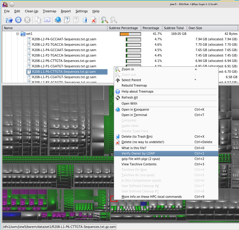
You can also use it to query files for what they are and most importantly, archive them in the background. See this separate doc for more information as to how to do this.
7. STDOUT, STDIN, STDERR, and Pipes
These are the input/output channels that Linux provides for communicating among your input, and program input and output
-
STDIN, usually attached to the keyboard. You type, it goes thru STDIN and shows up on STDOUT
-
STDOUT, usually attached to the terminal screen. Shows both your STDIN stream and the program’s STDOUT stream as well as …
-
STDERR, also usually connected to the terminal screen, which as you might guess, sometimes causes problems when both STDOUT and STDERR are both writing to the screen.
BUT these input & output channels can be changed to make data dance in useful ways.
There are several IO redirection commands:
-
> writes STDOUT to a file (ls -l /usr/bin > myfile)
-
< reads STDIN from file (wc < myfile)
-
>> appends STDOUT to a file (ls -l /etc >> myfile)
-
| pipes the STDOUT of one program to the STDIN of another program (cat myfile | wc)
-
tee splits the STDOUT and sends one of the outputs to a file. The other output continues as STDOUT. (ls -l /usr/bin | tee myfile2 | wc)
-
2> redirects STDERR to file
-
2>> appends STDERR to file
-
&> redirects BOTH STDERR and STDOUT to a file
-
2>&1 merges STDERR with STDOUT
-
2>&1 | merges STDERR with STDOUT and send to a pipe
-
|& same as 2>&1 | above
For example: ls prints its output on STDOUT. less can read either a file or STDIN. So..
# '|' is an anonymous pipe; connects the STDOUT of 'ls' to the STDIN of 'less'
ls -lt *.txt | less

# if we wanted to capture that output to a file as well..
ls -lt *.txt | tee alltxtfiles |less
While the above deals only with STDOUT and STDIN, you can also deal with STDERR in many confusing ways.
7.1. How to use pipes with programs
Here’s a simple example:
# What is the average size of the files in the directory '/data/apps/sources'?

# remember: 'ls -lR' will recursively list the long file listing, which contains
# the size in bytes so ...

ls -l /data/apps/sources |scut -f=4 | stats  # will tell you; try it

# and the following will plot the graph in a text-terminal
module load perl        # need to load a recent perl to provide modules needed by feedgnuplot
ls -l /data/apps/sources | scut -f=4 | feedgnuplot --terminal 'dumb'

# to expand the scale
ls -l /data/apps/sources | scut -f=4 | feedgnuplot --terminal 'dumb 100,40'

# or if you are running x2go or an X11 terminal, get the graphics version.
# and in this case, set the Y axis to log scale.
ls -l /data/apps/sources | scut -f=4 | feedgnuplot --extracmds 'set logscale y'
Here’s another. Break it up into individual commands and pipe each one into less to see what it produces, then insert the next command to see what it does
w |cut -f1 -d ' ' | sort | egrep -v "(^$|USER)" | uniq -c | wc

w | less
w |cut -f1 -d ' ' | less
w |cut -f1 -d ' ' | sort | less
w |cut -f1 -d ' ' | sort | egrep -v "(^$|USER)" | less
w |cut -f1 -d ' ' | sort | egrep -v "(^$|USER)" | uniq -c | less
Pipes allow you to mix and match output and input in various useful ways. Remember STDOUT/STDIN when you’re designing your own programs so you can format the output and read the input in useful ways down the road.
7.2. tee, subshells, and pipes.
As noted above, tee taps the STDOUT and sends one copy to a file (or set of files) and allows the other copy to continue to STDOUT. This allows you to duplicate the STDOUT to do all kinds of useful things to keep your data in flight.
tee is especially useful in conjunction with subshells - starting a new shell to process one branch of the tee while allowing the STDOUT to continue to other analyses. The use of subshells is one way to allow arbitrary duplication of output as shown below:
tar -czf - somedir  |  pv -trb | tee >(tee >(shasum > sha.file) | wc -c > wc.file)  > /dev/null

# what does this do?  What is /dev/null? How would you figure it out?
so the format is | tee >(some chain of operations), repeated as needed, including another tee. On the right side of the last ) is the STDOUT and you can process it in any way you’d normally process it.
7.3. The File Cache
When you open a file to read it, the Linux kernel not only directs the data to the analytical application, it also copies it to otherwise unused RAM, called the filecache. This assures that the second time that file is read, the data is already in RAM and almost instantly available. The practical result of this caching is that the SECOND operation (within a short time) that requests that file will start MUCH faster than the first. A benefit of this is that when you’re debugging an analysis by repeating various commands, doing it multiple times will be very fast.
8. Text files
Most of the files you will be dealing with are text files. Remember the output of the file command:
Sat Mar 09 11:09:15 [1.13 1.43 1.53]  hmangala@hpc:~/nco-4.2.5
566 $ file *
acinclude.m4: ASCII M4 macro language pre-processor text
aclocal.m4:   Ruby module source text
autobld:      directory
autogen.sh:   POSIX shell script text executable
bin:          directory
bld:          directory
bm:           directory
config.h.in:  ASCII C program text
configure:    POSIX shell script text executable
configure.eg: ASCII English text, with very long lines
configure.in: ASCII English text, with very long lines
COPYING:      ASCII English text
data:         directory
doc:          directory
files2go.txt: ASCII English text, with CRLF line terminators  <<<<
INSTALL:      ASCII English text
m4:           directory
Makefile.am:  ASCII English text
Makefile.in:  ASCII English text
man:          directory
obj:          directory
qt:           directory
src:          directory
Anything in that listing above that has ASCII in it is text, also POSIX shell script text executable is also a text file. Actually everything in it that isn’t directory is a text file of some kind, so you can read them with less and they will all look like text.
|
|
DOS EOLs
If the file description includes the term with CRLF line terminators (see <<<< above), it has DOS newline characters. You should convert these to Linux newlines with dos2unix before using them in analysis. Otherwise the analysis program will often be unable to recognize the end of a line. Sometimes even filenames can be tagged with DOS newlines, leading to very bizarre error messages. |
Text files are the default way of dealing with information on Linux. There are binary files (like .bam files or anything compressed (which a bam file is), or often, database files, and specialty data files such as netCDF or HDF5.
You can create a text file easily by capturing the STDOUT of a command.
In the example above, you could have captured the STDOUT at any stage by redirecting it to a file
# We use '/usr/bin' as a target for ls because if you do it in
# your own dir, the 1st command will change the file number of and size
# and result in a slightly different result for the second.
# '/usr/bin' is a stable dir that will not change due to this command.

ls -lR /usr/bin | scut -F=4 | stats

# could have been structured (less efficiently) like this:

ls -lR /usr/bin > ls.out
scut -F=4 < ls.out > only.numbers
cat only.numbers | stats

# note that '<' takes the STDOUT of the file to the right and directs it to
# the STDIN of the program to the left.
#  '>' redirects the STDOUT of the app to the left to the file on the right
# while '|' pipes the STDOUT of the program on the left to the program on the right.


# what's the diff between this line?

cat only.numbers > stats

# and this line:

cat only.numbers | stats

# Hmmmmm?
|
|
Files vs Pipes
When you create a file, a great many operations have to be done to support creating that file. When you use a pipe, you use fewer operations as well as not taking up any intermediate disk space. All pipe operations take place in memory, so are 1000s of times faster than writing a file. A pipe does not leave any trace of an intermediate step tho, so if you need that intermediate data, you’ll have to write to a file or tap the pipe with a tee. |
8.1. Viewing Files
8.1.1. Pagers, head & tail
less & more are pagers, used to view text files. In my opinion, less is better than more, but both will do the trick.
less somefile  # try it

alias less='less -NS' # is a good setup (number lines, scroll for wide lines)

# some useful head and tail examples.

head -XXX  file2view  # head views the top XXX lines of a file
tail -XXX  file2view  # tail views the bottom XXX lines of a file
tail -f    file2view  # keeps dumping the end of the file if it's being written to.
tail -n +XX file2view # views the file STARTING at line XX (omits the top (XX-1) lines)
8.1.2. Concatenating files
Sometimes you need to concatenate / aggregate files; for this, cat is the cat’s meow.
cat file2view                    # dumps it to STDOUT
cat file1 file2 file3 > file123  # or concatenates multiple files to STDOUT, captured by '>' into file123
8.2. Slicing Data
cut and scut allow you to slice out columns of data by acting on the tokens by which they’re separated. A token is just the delimiter between the columns, typically a space or <tab>, but it could be anything, even a regex. cut only allows single characters as tokens, scut allows any regex as a token.
# lets play with a gene expression dataset:
wget http://moo.nac.uci.edu/~hjm/red+blue_all.txt.gz

# how big is it?
ls -l red+blue_all.txt.gz

# Now lets decompress it
gunzip red+blue_all.txt.gz

# how big is the decompressed file (and what is it called?

# how compressed was the file originally?

# take a look at the file with 'head'
head red+blue_all.txt

# hmm - can you tell why we got such a high compression ratio with this file?

# OK, suppose we just wanted the fields 'ID' and 'Blue' and 'Red'
# how do we do that?

# cut allows us to break on single characters (defaults to the TAB char)
# or exact field widths.


# Let's try doing that with 'cut'

cut -f '1,4,5' <  red+blue_all.txt | less    # cuts out the fth field (counts from 1)

# can also do this with 'scut', which also allows you to re-order the columns
# and break on regex tokens if necessary..

scut -f='4 5 1' <  red+blue_all.txt   | less  # cuts out whatever fields you want;

# and also awk, tho the syntax is a bit  .. awkward
awk '{print $4"\t"$5"\t"$1}' < red+blue_all.txt | less

# note that the following produces the same output:
awk '{print $4    "\t"    $5   "\t"     $1}' < red+blue_all.txt | less
You might wonder why the output of the awk command is different than scut’s. The difference is in the way they index. awk and cut index from 1, scut indexes from 0. Try them again and see if you can make them output the identical format.
If you have ragged columns and need to view them in aligned columns, use cols to view data.
Or column. cols can use any Perl-compatible Regular Expression to break the data. column can use only single characters.
# let's get a small data file that has ragged columns:
wget http://moo.nac.uci.edu/~hjm/MS21_Native.txt

less  MS21_Native.txt  # the native file in 'less'

# vs 'column'
column < MS21_Native.txt | less  # viewed in columns

# and by 'cols' (aligns the top 44 lines of a file to view in columns)
# shows '-' for missing values.
cols --ml=44 < MS21_Native.txt | less   #
8.3. Rectangular selections
Many editors allow columnar selections and for small selections this may be the best approach Linux editors that support rectangular selection
| Editor | Rectangular Select Activation |
|---|---|
nedit |
Ctrl+Lmouse = column select |
jedit |
Ctrl+Lmouse = column select |
kate |
Shift+Ctrl+B = block mode, have to repeat to leave block mode. |
emacs |
dunno - emacs is more a lifestyle than an editor but it can be done. |
vim |
Ctrl+v puts you into visual selection mode. |
8.4. Finding file differences and verifying identity
Quite often you’re interested the differences between 2 related files or verifying that the file you sent is the same one as arrived. diff and especially the GUI wrappers (diffuse, kompare) can tell you instantly.
diff file1 file1a            # shows differences between file1 and file2
diff hlef.seq hlefa.seq      # on hpc, after changing just one base.

# can also do entire directories (use the nco source tree to play with this).
# Here we use 'curl' to get the file and unpack in in one line.
cd $DD
curl http://moo.nac.uci.edu/~hjm/nco-4.2.5.tar.gz | tar -xzf -

diff -r path/to/this/dir   path/to/that/dir > diff.out &

# 'comm' takes SORTED files and can produce output that says which line
# is in file 1, which is file 2 & which is in both.

ie:
comm  file1.sorted file2.sorted

# md5sum generates md5-based checksums for file corruption checking.

md5sum files           # lists MD5 hashes for the files
# md5sum is generally used to verify that files are identical after a transfer.
# md5 on MacOSX, <http://goo.gl/yCIzR> for Windows.

md5deep -r   # can recursively calculate all the md5 checksums in a directory
8.5. The grep family
grep sounds like something blobby and unpleasant and sort of is, but it’s VERY powerful. It’s a tool that uses patterns called Regular Expressions to search for matches.
8.5.1. Regular Expressions
Otherwise known as regexes, these are the most powerful tools in a type of computation called string searching and for researchers, a huge help in data munging and cleansing.
They are not exactly easy to read at first, but it gets easier with time.
The simplest form is called globbing and is used within bash to select files that match a particular pattern
ls -l *.pl      # all files that end in '.pl'
ls -l b*.pl     # all files that start with 'b' & end in '.pl'
ls -l b*p*l     # all files that start with 'b' & have a 'p' somewhere & end in 'l'
There are differences between globbing (regexes used to identify files) and regex matching to look for patterns inside of files. Here’s a good article that differentiates between the 2.
Looking at nucleic acids, can we encode this into a regex?:
gyrttnnnnnnngctww = g[ct][ag]tt[acgt]{7}gct[at][at]
What if there were 4 to 9 'n’s in the middle?
gyrttnnnnnnngctww = g[ct][ag]tt[acgt]{4,9}gct[at][at]
grep regex files    # look for a regular expression in these files.

grep -rin regex  *  # recursively (-r) look for this case-INsensitive (-i) regex
                    # in all files and dirs (*) from here down to the end and
                    # prefix the match line with the line number.

grep -v regex files # invert search (everything EXCEPT this regex)

grep "this\|that\|thus" files # search for 'this' OR 'that' OR 'thus'

egrep "thisregex|thatregex" files  # search for 'thisregex' OR 'thatregex' in these files

#ie
egrep "AGGCATCG|GGTTTGTA" hlef.seq
If you want to grab some sequence to play with, here’s the Human Lef sequence.
|
|
Regexes and biosequences
Note that these grep utilities won’t search across lines unless explicitly told to, so if the sequence is split AGGC at the end of one line and ATCG at the beginning of another, it won’t be found. Similarly, the grep utilities won’t search the reverse complement. For that you’ll need a special biosequence utility like tacg or Bioconductor (both installed on HPC). |
This is a pretty good quickstart resource for learning more about regexes. Also, if you’re using x2go to export a terminal session from HPC, and have a choice of terminals to use, gnome-terminal allows searching in text output, but not as well as konsole.
9. Info About (& Controlling) your jobs
Once you have multiple jobs running, you’ll need to know which are doing what. Here are some tools that allow you to see how much CPU and RAM they’re consuming.
jobs           # lists all your current jobs on this machine
qstat -u [you] # lists all your jobs in the SGE Q
[ah]top  # lists the top CPU-consuming jobs on the node

ps       # lists all the jobs which match the options
ps aux   # all jobs
ps aux | grep hmangala  # all jobs owned by hmangala
ps axjf                 # all jobs nested into a process tree
pstree   # as above

alias psg="ps aux | grep"  # allows you to search processes by user, program, etc

kill -9 JobPID#   # kill off your job by PID
To practice, let’s get a source code
9.1. Background and Foreground
Your jobs can run in the foreground attached to your terminal, or detached in the background, or simply stopped.
Deep breath…..
-
a job runs in the foreground unless sent to the background with & when started.
-
a foreground job can be stopped with Ctrl+z (think zap or zombie)
-
a stopped job can be started again with fg
-
a stopped job can be sent to the background with bg
-
a background job can be brought to the foregound with fg
-
normally, all foreground & background & stopped jobs will be killed when you log out
-
UNLESS your shell has been configured to allow these processes to continue by setting the shell option shopt settings to allow it. On HPC we have done that for you so background jobs will continue to run (shopt -u huponexit).
-
OR UNLESS you explicitly disconnect the job from the terminal by prefixing it with nohup. ie
nohup some-long-running-command
If you were going to run a job that takes a long time to run, you could run it in the background with this command:
tar -czf gluster-sw.tar.gz gluster-sw  &
# The line above would run the job in the background immediately and notify
# you when it was done by printing the following line to the terminal
...
[1]+  Done                    tar -czvf gluster-sw.tar.gz gluster-sw

tar -czvf gluster-sw.tar.gz gluster-sw &  #  What's wrong with this command?
#      ^  .. hint
HOWEVER, for most long-running jobs, you will be submitting the jobs to the scheduler to run in batch mode. See here for how to set up a qsub run.
10. Finding files with find and locate
Even the most organized among you will occasionally lose track of where your files are. You can generally find them on HPC by using the find command. find is a very fast and flexible tool, but in complex use, it has some odd but common problems with the bash shell.
# choose the nearest dir you remember the file might be and then direct 'find' to use that starting point
find [startingpoint] -name filename_pattern

# ie:  (you can use globs but they have to be 'escaped' with a '\'
# or enclosed in '' or "" quotes
$ find gluster-sw/src -name config\*
gluster-sw/src/glusterfs-3.3.0/argp-standalone/config.h
gluster-sw/src/glusterfs-3.3.0/argp-standalone/config.h.in
gluster-sw/src/glusterfs-3.3.0/argp-standalone/config.log
gluster-sw/src/glusterfs-3.3.0/argp-standalone/config.status
gluster-sw/src/glusterfs-3.3.0/argp-standalone/configure
gluster-sw/src/glusterfs-3.3.0/argp-standalone/configure.ac
gluster-sw/src/glusterfs-3.3.0/xlators/features/marker/utils/syncdaemon/configinterface.py

# this is equivalent:
find gluster-sw/src -name 'config*'
You can also use find to do complex searches based on their names, age, etc.
Below is the command that finds
-
zero sized files (any name, any age)
-
files that have the suffix .fast[aq], .f[aq], .txt, .sam, pileup, .vcf
-
but only if those named files are older than 90 days (using a bash variable to pass in the 90)
The -o acts as the OR logic and the -a acts as the AND logic. Note how the parens and brackets have to be escaped and the command is split over multiple lines with the same backslash, but note that at the end of a line, it acts as a continuation character, not an escape. Yes, this is confusing.
DAYSOLD=90
find .  -size 0c \
        -o \( \
        \( -name \*.fast\[aq\] \
        -o -name \*.f\[aq\]  \
        -o -name \*.txt  \
        -o -name \*.sam  \
        -o -name \*pileup \
        -o -name \*.vcf \) \
        -a -mtime +${DAYSOLD} \)
locate is another very useful tool, but it requires a full indexing of the filesystem (usually done automatically every night) and will only return information based on the permission of the files it has indexed. So you will not be able to use it to locate files you can’t read.
In addition, locate will have limited utility on HPC because there are so many user files that it takes a lot of time and IO to do it. It is probably most useful on your own Linux machines.
# 'locate' will work on most system files, but not on user files. Useful for looking for libraries,
# but probably not in the module files

locate libxml2 |head   # try this

# Also useful for searching for libs is 'ldconfig -v', which searches thru the LD_LIBRARY_PATH

ldconfig -v |grep libxml2
11. Modules & searchmodules
Modules (actually Environment Modules) are how we maintain lots of different applications with multiple versions without (much) confusion. The basic commands are:
module load app          # load the numerically highest version of the app module
module load app/version  # load the module with that specific version
module whatis app        # what does it do?
module avail bla         # what modules are available that begin with 'bla'
module list              # list all currently loaded modules
module rm app            # remove this module (doesn't delete the module,
                         #   just removes the paths to it)
module unload app        # same as 'rm' above
module purge             # removes ALL modules loaded (provides you with a
                         #   pristine environment; strongly advised in a script
HINT: to be able to page thru the modules and search the names, use this alias:
alias modav='module avail 2>&1 >/dev/null | less'
The reason for the inclusion of the 2>&1 >/dev/null is that the module commands send output to STDERR, not STDOUT. See why this is important above.
In order to find the module you want, you can either use the appropriate module command or use searchmodules (HPC-specific) to search through not only all modules, but all sub-modules which have been installed in Perl, Python, and R.
$ module avail R       # search for all modules that begin with 'R' (case-sensitive).

---------------------- /data/modulefiles/SOFTWARE -----------------------
R/2.14.0          R/3.1.1           R/3.4.1           Ray/2.3.1
R/2.14.2          R/3.1.2(default)  R/3.5.1           RevolutionR/5.0.1
R/2.15.0          R/3.1.3           R/3.5.3           RNAcode/0.3

[etc]


$ module avail -l R    # provide the date of installation; useful to see which one is latest.

- Package -----------------------------+- Versions -+- Last mod. ------
/data/modulefiles/SOFTWARE:
R/2.14.0                                             2017/07/09 21:11:56
R/2.14.2                                             2017/07/09 21:11:56
R/2.15.0                                             2017/07/09 21:11:56
R/2.15.1                                             2017/07/09 21:11:56
R/2.15.2                                             2017/07/09 21:11:56
R/3.0.1                                              2014/05/02 22:40:28

[etc]
But searchmodules allows searching thru the submodules and will return the versions thereof. Note that torch occurs in several Python/anaconda modules, as well as in R.
$ searchmodules torch
anaconda/2.7-4.3.1            torch                         0.4.1
anaconda/2.7-4.3.1            torchvision                   0.2.1
anaconda/3.5-2.4.0            torch                         0.1.11+b13b701
anaconda/3.5-2.4.0            torchvision                   0.1.8
anaconda/3.6-5.0.1            torch                         1.0.0
anaconda/3.6-5.0.1            torch-encoding                1.0.1
anaconda/3.6-5.0.1            torchtext                     0.2.3
anaconda/3.6-5.0.1            torchvision                   0.2.1
anaconda/3.7-5.3.0            torch                         1.0.1
python/2.7.15                 torch                         0.4.1
python/2.7.15                 torch-vision                  0.1.6.dev0
python/2.7.15                 torchvision                   0.2.1
R/3.1.3                       blowtorch                     1.0.2
R/3.2.2                       blowtorch                     1.0.2
In order to load a particular module, you have to call it up with the specific version if you don’t want the latest one.
Note that the latest one may not be the numerically largest one. Many packages (including Linux) number their packages such that 2.6.16 is newer than 2.6.3 (but older than 2.6.30).
12. Getting files from the web
12.1. Checksums
A checksum is a single long string that encodes the integrity of an file. If a single bit changes in the file, the checksum will change as well. There are a number of algorithms to calculate checksums, varying in strength and ability to encode various sizes of files, but generally the MD5 checksum is still used a lot. When you’re generating output, you should also generate a checksum log of the output files and email it to yourself (as well as storing it on HPC) to enable you verify the integrity of the file later on, say after a filesystem hiccup.
The current general purpose checksum program is hashdeep (md5deep is the same program). When invoked on a single file, it will by default produce the MD5 and SHA-256 hashes, along with some invocation info and the name of the file. As the deep part implies, it can also do recursive checksumming if you give it the -r flag (good for generating checksums on an entire output directory) and if saved to a file, can easily be emailed or used to compare after a suspicious event (it will read the file and compare all the new checksums to the old checksums in the file.
$ hashdeep Linux_Tutorial_12.html
%%%% HASHDEEP-1.0
%%%% size,md5,sha256,filename
## Invoked from: /home/hjm/nacs
## $ hashdeep Linux_Tutorial_12.html
##
261699,8716b0279f50a417790a20844aceea5e,bcecb4e3fce8484c22da43a5071524b3a3a961efdfcd3f0ab5e53523cd9ea0b6,/home/hjm/nacs/Linux_Tutorial_12.html

# Now I change one character from 9 -> 8, so the bytecount is identical

$ hashdeep Linux_Tutorial_12.html
%%%% HASHDEEP-1.0
%%%% size,md5,sha256,filename
## Invoked from: /home/hjm/nacs
## $ hashdeep Linux_Tutorial_12.html
##
261699,d2cccc70c1173e7c41598a0074e5e99b,60ba97ab64a783d9d66afd952e3f7127ac636a551872ce4084578c53f5195298,/home/hjm/nacs/Linux_Tutorial_12.html

# note that both MD5 and SHA-256 hashes are completely different, even tho the bytecount is identical
# 261699,8716b0279f50a417790a20844aceea5e,bcecb4e3fce8484c22da43a5071524b3a3a961efdfcd3f0ab5e53523cd9ea0b6
# 261699,d2cccc70c1173e7c41598a0074e5e99b,60ba97ab64a783d9d66afd952e3f7127ac636a551872ce4084578c53f5195298
# ^^^^^^
For complete directory tree, the effect is similar:
# get a fresh copy of the nco source file: (see the 'curl' section immediately below)
# and unpack it.
curl http://moo.nac.uci.edu/~hjm/biolinux/nco/nco-4.2.5.tar.gz | tar -xzf -

# it unpacks into a dir called 'nco-4.2.5'
ls  nco-4.2.5# as a reminder of what's here
COPYING   Makefile.am   aclocal.m4   bin/  config.h.in   configure.eg~  doc/  obj/
INSTALL   Makefile.in   autobld/     bld/  configure*    configure.in   m4/   qt/
INSTALL~  acinclude.m4  autogen.sh*  bm/   configure.eg  data/          man/  src/

# now run hashdeep on the whole directory recursively, capturing the output into a file
hashdeep -r nco-4.2.5 > nco.hashdeep

# and take a look at it:
head nco.hashdeep
%%%% HASHDEEP-1.0
%%%% size,md5,sha256,filename
## Invoked from: /home/hjm/nacs
## $ hashdeep -r nco-4.2.5
##
6137,fcb9681567452c897bdc76e2b745e06f,e714874d10fd1d0828728ebbfa580d976e7fa51010a250c4a9ab244e0e47ae84,/home/hjm/nacs/nco-4.2.5/bld/ddd_mpd.py
7109,1eae088275ae2dcb1f11ac7857f0aafe,bc26cf22b76a5ab750e3c95626570398cc3208ba7f108fc2d2c82b9a5b7e0c5c,/home/hjm/nacs/nco-4.2.5/bld/pvmgetarch
8777,8497c3702ed57378f1fd569ddbd75bd7,204cf85ede4145cee33dea5a9a12e8140421e0482626edfecb4efb09bdefa9c1,/home/hjm/nacs/nco-4.2.5/bld/nco.spec
936,9748d81fa6c9a925fa3186a5e141b8ae,dba79aaff8d9e6dd691ca21ee4e02685d8d994ad7dae3c8a5987a19a09664532,/home/hjm/nacs/nco-4.2.5/bld/pbuilder-sid
...

# now slightly modify a file.

joe nco-4.2.5/configure.in

# now check the file hashes against themselves with the files you just modified:
hashdeep -r -a -k nco.hashdeep nco-4.2.5
hashdeep: Audit failed

# hmm - which file file failed the audit?
hashdeep -r -x -k nco.hashdeep nco-4.2.5
/home/hjm/nacs/nco-4.2.5/configure.in   # bingo.

If you had a backup copy, you tell exactly WHERE the changes had happened as well with 'diff'
12.2. Graphical File Transfer tools
There are a number of ways to transfer files over networks. For beginners, GUI programs like those shown allow drag’n'drop file transfer between panes of the application.
As you get more advanced and want to do more things from the commandline, you’ll tend to use more of the tools listed below.
12.3. wget
wget will retrieve ftp or http URLs with a minimum of fuss, continuing a failed retrieval, creating a new name if a file already exists, and supporting a huge number of other options. It is used only for getting not putting. files, but as such, it’s a great choice to pull data files from Internet repositories.
wget http://moo.nac.uci.edu/~hjm/biolinux/nco/nco-4.2.5.tar.gz

# now get it again.
wget http://moo.nac.uci.edu/~hjm/biolinux/nco/nco-4.2.5.tar.gz  # when outside HPC

# what happened?
12.4. curl
Do everything in one line with curl. curl downloads the given URL and by default spits the whole thing to STDOUT, so this is a case where pipes (|) are meant to be used.
curl http://moo.nac.uci.edu/~hjm/biolinux/nco/nco-4.2.5.tar.gz | tar -xzf -

# tar's '-f' option means 'the following', and '-' typically means either STDOUT or STDIN,
# depending on context. So  'tar -xzf - ' means perform the tar magic on STDIN.

# if we wanted to know WHAT was being extracted, we could use the 'v' option like this:

curl http://moo.nac.uci.edu/~hjm/biolinux/nco/nco-4.2.5.tar.gz | tar -xzvf -

#                                                                   ^
13. Getting files from specific accounts
13.1. commandline scp (Mac, Linux, NOT Windows)
From your own laptop try to copy a file to HPC
scp TheFile You@hpc.oit.uci.edu:~
Did it appear to transfer? Where is it? Is it the right size? How do you tell?
# how many characters, words, and lines a file has.  Useful for text.
wc     file

# how many bytes are in a file
ls -l  file

# how big a file is in human-readable terms.
ls -lh file

# the md5 hash of a file (tests if files are identical).
md5sum file

# tells you which lines differ and where (also meld, kompare)
diff   file1 file2

# tells you how 2 dirs differ and where
diff -r dir1 dir2
13.2. commandline rsync (Mac, Linux)
Again, rsync is one of the most useful, efficient utilities for moving data that you’ll find. There are GUI versions for all platforms, and every MacOSX and Linux distro comes with the commandline version.
Let’s copy the entire AnalysisDir from your laptop to HPC (where AnalysisDir is some fairly small, readable dir that you choose).
rsync -av AnalysisDir You@hpc.oit.uci.edu:~
Now create a file in your LOCAL (laptop) AnalysisDir
ls -lat > AnalysisDir/listing
Now re-rsync
rsync AnalysisDir You@hpc.oit.uci.edu:~
See what happens?
13.2.1. Beware rsync’s delete option
Beware the --delete option with rsync. There are a lot of delete options with rsync:
   --del                   an alias for --delete-during
   --delete                delete extraneous files from dest dirs
   --delete-before         receiver deletes before xfer, not during
   --delete-during         receiver deletes during the transfer
   --delete-delay          find deletions during, delete after
   --delete-after          receiver deletes after transfer, not during
   --delete-excluded       also delete excluded files from dest dirs
   --ignore-missing-args   ignore missing source args without error
   --delete-missing-args   delete missing source args from destination
   --ignore-errors         delete even if there are I/O errors
   --force                 force deletion of dirs even if not empty
   --max-delete=NUM        don't delete more than NUM files
and some of them are REALLY dangerous (dropping-out-of-grad-school-dangerous). Be very aware what computer you’re on and what you’re doing and experiment on a junk directory before you and always use the -n flag (fake it first), before you do it for real.
The usual reason for using the --delete option is to force a complete sync operation between 2 computers, but the --delete option only works on the TARGET. So if you want to force this to sync your HPC dirs to your laptop (for example), you have to use your laptop as the target. Which means that you have to specify your laptop’s domain name or IP number, which changes at every new wireless location in UCI. There are certainly ways to determine this:
-
On MacOSX, Preferences → Sharing → Remote login (checked) will show the name that you have to use to login to your Mac.
-
on Linux, on wireless, this should work
ifconfig | grep -A1 "wlan\|wlp"| grep inet | cut -f2 -d: | cut -f1 -d' '
-
on Windows, try the following in a cmd window:
ifconfig | grep -A1 "wlan\|wlp"| grep inet | cut -f2 -d: | cut -f1 -d' '
The easiest approach may simply be to type "what is my IP " in a google search bar. That will almost always return your public IP number (which may NOT be your laptop’s IP (since if you’re at home, the public IP# is that of your wifi router). If you’re on-campus, it should be valid tho.
13.3. sshfs
sshfs is a mechanism that allows you to connect your laptop’s disk to a remote server (like HPC) or vice-versa. This is an incredibly useful mechanism to enable bi-directional data transfer relatively quickly and easily. Since it use your ssh connection, all the data passing back and forth is encrypted.
# from your laptop
cd
mkdir hpc
sshfs you@hpc.oit.uci.edu:/data/users/<your_UCINETID> ~/hpc

# enter password if prompted.  Let us know if it doesn't work. Then...
ls hpc

# don't for get to UNmount it WHEN YOU'RE DONE with the session.
# on your laptop:
fusermount -u ~/hpc

# if you're mapping your laptop's disk to your HPC account, you will probably
# have to map IDs with the option '-o uid=<UID>,gid=<GID>.
# ie get your HPC UID/GID with

id $USER

# then use that UID/GID to mount your laptop:

mkdir <HPC_mountpoint>
sshfs   -o uid=785,gid=200  hjm@<laptop_IP#>:<laptop_dir>  <HPC_mountpoint>
Once you’ve sshfs-mounted your HPC dir on your laptop, you can copy files back and forth, or edit them with your Mac editors to HPC as if it was on your laptop. Be sure to save eveything as plaintext.
You can also mount it the other way (mount your laptop to HPC) but often your laptop will have a DHCP address, so it may be trickier.
If you want to try this, it’s described in more detail here
13.4. Moving BigData
For bulk transfer of terabyte data, I’ve also written another document called How to transfer large amounts of data via network. And before you decide to download Wikipedia or the Library of Congress, please check in with us.
14. File Archives - tar and zip
14.1. tar
tar is (still) the default archive type for Linux/Unix. It creates a single file that contains everything that it’s pointed to, which provides some packing efficiency, and especially when it is explicitly compressed, a tar file will take only 30-50% of the original storage for generic text or sequence data, 1/20th the space for XML. tar by itself does not compress or decompress, but with the z, j, or J options, it can call de/compression routines on the tar file as it progresses.
tar -czvf tarfile.gz files2archive   # create a gzip'ed 'tarball'
tar -tzvf tarfile.gz                 # list the files in a gzip'ed 'tarball'
tar -xzvf tarfile.gz                 # extract a gzip'ed 'tarball'
tar -xzvf tarfile.gz  included/file  # extract a specific 'included/file' from the archive.
Also, consider archivemount to manipulate files while still in a tarball.
14.2. zip
Zip comes from the PC world’s pkzip. The format is now standardized and files zipped on PCs and Macs can be handled by the Linux zip/unzip. Because Windows users and utilities are more used to zip archives, they are often used to punt data back and forth to Windows.
zip zipfilename files2archive        # zip the 'files2archive' into the 'zipfilename'
unzip -l zipfilename.zip             # list the files that are in zipfilename.zip without unzipping them
unzip  zipfilename.zip               # unzip the 'zipfilename.zip' archive into the current dir.
Let’s try to zip that nco directory with zip
cd
zip nco_src nco-4.2.5

# how big is it?
# how big is the gzipped version?
# how do you tell?
15. Compression Utilities
15.1. gzip/gunzip
The gzip family is probably the most popular de/compression utility on Linux. It will reduce the size of a sequence file to about 30% of the original.
gzip somefile  # will result in only the compressed file - 'somefile.gz'
gunzip nco-4.2.5.tar.gz   # to DEcompress the file -> nco-4.2.5.tar

# or could use 'pigz' for parallel de/compression on multi-core machines
pigz -p4 chr1.fa  # compresses this file using 4 cores in parallel
Only use pigz on files over ~1GB bc the overhead takes time to set up and monitor. pigz is fantastic but for small files, it won’t make much difference; for large multiGB files it will.
15.2. bzip2/bunzip2
The other major de/compression tool on Linux is called bunzip2 and is slightly more efficient, and slightly slower than gzip. It also has a parallel equivalent called pbzip2, which is also installed on HPC.
There are lots of compression utilities. Use Google to find the most appropriate one.
15.3. archivemount
archivemount is a utility to mount compressed archives as filesystems, so instead of leaving a cloud of ZOTfiles behind you, use tar or zip to compress them all into one archive and then interact with them via archivemount.
16. VERY simple bash programming
bash is not only the shell with which you interact when you log onto HPC, it’s also a fully functional (if ugly) Turing complete programming language. Using the simple features can make you very productive. Trying to use the advanced features will make you very unproductive. Learn to use Perl or Python instead. There are 1000’s of pages of bash help available. Here’s a good one. And here’s another - the Pure Bash Bible.
16.1. bash variables
Remember variables from math? A variable is a symbol that can hold the value of something else. In most computer languages (including bash) a variable can contain:
-
numeric values like: +156, 83773.34, 3.5e12, -2533
-
strings like: "booger", "nutcase","24.334" (a string, not a number when quoted) "and even this phrase"
-
lists or arrays like:
-
[12 25 64 98735 72]
-
[238.45 672.6645 0.443 -51.002]
-
["if" "you" "have" "to" "ask" "then" "maybe" "…"]
-
Note that in lists or arrays, the values are of the same type (integers, floats, strings, etc). Most languages also allow the use of more highly complex data types (often referred to as data structures, objects, dataframes, etc). Even bash allows you to do this, but it’s so ugly that you’d be better off gouging out your own eyeballs. Use one of Perl, Python, R, Java, etc.
All computer languages allow comments. Often (bash, perl, python, R) the comment indicator is a "#" which means that anything after the "#" is ignored, even if it’s not the 1st character in a line. This allows you to comment out later parts of a line if you’re testing a command by inserting the "#" where you want the command to be ignored.
Here are some examples of variables in bash.
thisvar="peanut"    # note the spacing
thisvar = "peanut"  # what happened?  In bash, spacing/whitespace matter

thatvar="butter"

echo thisvar

# ?? what happened? Now..

echo $thisvar  # what's the difference?

thisvar='hazelnut'         # now try it with single quotes

echo $thisvar              # does it work as expected?

echo "$thisvar"            # does this do what you want?

echo '$thisvar'            # does this?  What's the difference?

echo "'$thisvar'"          # and what about this? Surprising?

echo '"$thisvar"'          # and if we switch the order of the quotes?

echo "'"$thisvar"'"        # and start stacking quotes?

# NB: If a variable seems to behave oddly, and nothing else explains the
# misbehavior, you're probably quoting it wrong
# single and double quoting also have different effects on regular expressions
# in strings.

###  SO BE CAREFUL WITH QUOTING.   ###

# note that in some cases, you'll have to protect the variable name with {}

echo $thisvar_$thatvar      # what's the difference between this

echo ${thisvar}_${thatvar}  # and this?
You can use bash variables to present the results of system commands if they’re inside of parens ():
seq 1 5  # what does this do?

filecount=$(seq 1 5)
echo $filecount  # what's the difference in output?


dirlist=$(ls -1) # the same thing happens here.
echo $dirlist
You can also assign multiple variables at a time from an argument or command.
# if you wanted to capture the 3 variables marked below:
df -h /
Filesystem      Size  Used Avail Use% Mounted on
/dev/sda1        59G   14G   43G  24% /
                 ***   ***   ***
You could execute 3 commands to extract the one by one:

Size=`df -h / | grep -v Filesystem | awk '{printf  $2}'`
Used=`df -h / | grep -v Filesystem | awk '{printf  $3}'`
Avail=`df -h / | grep -v Filesystem | awk '{printf  $4}'`

echo $Size $Used $Avail
59G 14G 43G

# or you could capture them all at once with:
read -r  Size Used Avail <<< `df -h / | grep -v Filesystem | awk '{ print  $2,$3,$4}'`
echo $Size $Used $Avail
59G 14G 43G
16.2. Escaping characters
Occasionally, you’ll come across a situation where you’ll have to escape a character in order to get the bash shell to recognize it as the character you want. The most frequent example of this is with embedded spaces in filenames. The bash shell needs to know what the name of a file is. The standard is to use spaces to separate filenames and parts of commands. So if you try to process a file from Windows called "RNASeq data from 2018" on the commandline, the shell will perceive it as 4 files, not 1; the embedded spaces will cause confusion.
One way to deal with this problem is to replace the spaces with underscores (_) before copying it to a Linux system. However, if you don’t replace the spaces, once it’s on the Linux system you can still manipulate it, but you’ll have to prefix the spaces with a "\" to escape the character. ie tell the shell that the escaped character is part of the filename string, not the separation token.
So if you wanted to use the Windows-filename-with-spaces on Linux without changing the name, you can either protect the individual spaces with "\" or protect the entire filename with single or double quotes as shown above with "RNASeq data from 2018".
mv RNASeq\ data\ from\ 2018 RNASeq_data_from_2018
# or
mv "RNASeq data from 2018" RNASeq_data_from_2018
In both the above cases, you’re protecting the space from being interpreted as a separation token.
This is also seen with leading tildes (~), which some editors use to name backup copies. The tilde is more frequently used to denote HOME directories, so unless you escape it, the shell will try to interpret it as the name of someone’s HOME.
Other characters often need to be escaped in scripting languages to prevent being interpreted as variable names (chiefly bash and Perl with the $ character.)
16.3. Flattening results
By default, bash will flatten results, deleting newlines (aka \n) and returning flat lists of values in a single line as values which is useful in file name processing. Sometimes you want to maintain the newlines. To do that, you can double-quote the variable which will maintain the newlines.
ls  # note how wide the default printing is
2014-April.txt   2014-February.txt  2014-July.txt  2014-March.txt  2014-September.txt
2014-August.txt  2014-January.txt   2014-June.txt  2014-May.txt

yy=`ls`  # feed the output of 'ls' into the variable 'yy'

echo $yy # note that the output is a continuous line of the above output w/ no newlines.
2014-April.txt 2014-January.txt 2014-March.txt 2014-August.txt 2014-July.txt 2014-May.txt 2014-February.txt 2014-June.txt 2014-September.txt

echo "$yy"  # with $yy in double-quotes, the newlines are retained.
2014-April.txt     2014-January.txt  2014-March.txt
2014-August.txt    2014-July.txt     2014-May.txt
2014-February.txt  2014-June.txt     2014-September.txt

# and of course, if $yy is in single quotes, you only get back the *literal* $yy
echo '$yy'
$yy
|
|
Debugging bash
As noted, bash is a good job control language, but a lousy formal programming language. To debug a bash script, besides inserting loads of echo commands, you can also use the "-x" flag which will announce every command and the result. Because the "-x" output can be egregiously verbose, you can also fencepost the debugging by enclosing the the code to be debug with " set -x" as described here in more detail There is also now a free full-featured bash debugger available for complex bash scripts. This is how it works. |
16.4. Math in bash
Well, it’s ugly. Native bash math is integer math, meaning that manipulation of decimal fractions is ignored or forbidden. The spacing between variables is also important, unlike many languages. There are 2 ways to manipulate integers in bash natively. The 1st is with the expr prefix; the 2nd is with the let prefix. Some examples:
# return the sum of 2 integers
expr 12 + 13
25             # which is expected

# but change the spacing and the result:
expr 12+13
12+13          # might not be expected.

# remember, it's INTEGER-ONLY math
expr 12.5 + 13.5
expr: non-integer argument

# similarly to assign to a variable WITHOUT "let"

rr=12+13  # no error on the assignment, but ..
echo $rr
12+13     # you get the literal string back, not the expected sum

# to assign to the variable, you have to use 'let'
let rr=12+13
echo $rr
25         # ok, but note the spacing
# if you relax the spacing, you get errors.
let rr=12 + 13
bash: let: +: syntax error: operand expected (error token is "+")

# if you enclose the expression in quotes, you might expect to get a string back
# but in fact, it works as math.  Go figure..

let rr="12 + 13"
echo $rr
25

# it's INTEGER math

let rr=25/5
echo $rr
5        # fine.  but note that
let rr=29/5
echo $rr
5        # also equals 5, bc bash *truncates* fractional math
16.4.1. For bash math, use bc instead
To extract somewhat rational behavior from bash, use gnu bc (binary calculator) which is distributed with all linux distros. You have to set the precision, and then send the expression to bc. It looks ugly (and is), but it’s better than bash.
num=48.373     # sets 'num' as a string
denom=58.22    # ditto for 'denom'
# then set the decimal precision with 'scale' and feed the expression into 'bc'
# note the `backtics`
frac=`echo "scale=4;$num/$denom" | /usr/bin/bc`
echo $frac
.8308  # the result a normal human would want.

# also, spacing is not as much as a concern; compare with the line above
frac=`echo "scale = 4; $num / $denom" | /usr/bin/bc`
echo $frac
.8308  # it's still the same value
See "man bc" for all the things "bc" can do.
16.5. Looping with bash
Simple bash loops are very useful
# this loop will output all the lines that contain 'the' in all files
# ending in '.txt'
for file in *.txt; do
   grep 'the' $file
done
You can also trap the output of a loop’s individual commands into a single STDOUT stream to process with another command by enclosing the loop in parens (). ie, process all of the individual outputs as a single output.
# as above, the for loop will output all the lines that contain 'the'
# in all files ending in '.txt' but all those characters will be passed
# thru 'wc' to count the number of chars, words, & lines.

(for file in *.txt; do
   grep 'the' $file
done) | wc
16.5.1. The bash line eater
Bash is a horrible language and you shouldn’t be doing this kind of thing using bash, but sometimes it’s more useful than breaking into Python, Perl, R, Julia, etc.
The setup is if you want to read a file, line by line, then do something with each line. The following microprogram reads filename one line at a time and then emits the line in the format specified by the echo line.
Also, beware the IFS (Internal Field Separator), normally whitespace.
ORIGIFS=$IFS
FILE=outreach.karyo.txt # set to a text file name
N=0
while read LINE; do
    let N=$N+1 # 'N' must be assigned as a 'naked' name, not a $variable
    echo "Input line [$N] is: [$LINE]"
    # read -ra array <<< "$LINE"
    array=( $LINE )
    for ii in $(seq 1 5); do echo "[$ii]:[${array[$ii]}]  "; done
    sleep 2
done  <  $FILE
If you start messing with IFS, don’t forget that
unset IFS
will get yo uback to the original default condition.
16.6. Iterating with loops
for outer in $(seq 1 5); do
  for inner in  $(seq 1 2); do
    # try this with and without variable protection
    echo "processing file bubba_${inner}_${outer}"
  done
done
16.7. Strings in bash
A string in bash is much like in other languages, an array of characters
# assigning string vars
wordstring="this is a string"
alsostring="254.98752"
longerstring="the rain in spain falls mainly on the plain"

# get length of string
echo ${#wordstring}
echo ${#alsostring}
echo ${#longerstring}

# how to take substrings
echo ${wordstring:4}  # the '4' marks the beginning of the substring
echo ${wordstring:2}

# when there are 2 numbers, the 2nd (':6') denotes the length of
# the substring to return
echo ${longerstring:12:6}

# the 2nd can also be negative, demoting that the count is from the end
# towards the beginning
echo ${longerstring:12:-6}

# see the difference between the 2 terms above?

echo ${#longerstring}  # how long is $longerstring?
# what do you think is going to happen in the command below?
for bb in $(seq 0 33); do echo ${longerstring:$bb:24}; done
# why did it do that?


# can also use vars to define the offsets
bgn=10
off=16
# reference strings as:  string:begin:offset
echo ${longerstring:$bgn:$off}

# using vars to cycle
for bb in $(seq 0 33); do
  let ee="$bb + 6"; echo "$bb - $ee"; echo ${longerstring:$bb:$ee};
done

# did you notice how we calculated the new value (math in bash is ugly).
16.8. Stream-editing
As you may have noticed by this time, one of the enormous advantages that Linux offers is the ability to process data in a stream with the STDOUT/STDIN/STDERR channels. As well as filtering data in streams with tools like grep, cut/scut, join, etc, you can also change the values of the stream as well. Below is a tiny example of some approaches to changing text in a stream. The easiest way to solve your particular stream editing problem is to Google for the solution, but the examples below give you a sense of how the different options work.
16.8.1. tr
tr is used to translate (or delete) single characters. Quite often you need to modify single characters and this is a simple, easy-to-remember command to do that.
input="abcdefg"
echo $input | tr -d 'c'  # deletes a char
abdefg

echo $input | tr -d'c' # this won't work.  why not?

echo $input | tr 'c' 'z'  # translates a char
abzdefg

# can also use tr to operate on case of characters as well
input="The Rain in Spain Falls Mainly On The Plain"
echo $input | tr '[:lower:]' '[:upper:]'
THE RAIN IN SPAIN FALLS MAINLY ON THE PLAIN

# you can chain 'tr' operations to do multiple things in the same operation.
input="The Rain in Spain Falls Mainly On The Plain"
echo $input | tr '[:lower:][:upper:]' '[:upper:][:lower:]'
tHE rAIN IN sPAIN fALLS mAINLY oN tHE pLAIN
See the Wikipedia entry and Google for other examples.
16.8.2. sed
sed (for stream editor) is the big brother of tr. You can use sed to do almost any stream-based text manipulation. The downside is that it’s more complicated to use. Below are some simple examples.
The usual use of sed is to apply it on a file or large stream of STDIN, such as:
sed 's/regexp/replacement/g' inputFileName > outputFileName
but in the examples below, I use the output from an echo command for brevity.
input="The Rain in Spain Falls Mainly On The Plain"
echo $input | sed 's/Spain/Greece/'
The Rain in Greece Falls Mainly On The Plain

# however.. note below
input="The Rain in Spain Falls Mainly On The Plain of Spain"
echo $input | sed 's/Spain/Greece/'
The Rain in Greece Falls Mainly On The Plain of Spain
# note that only the 1st 'Spain' is converted.

input="The Rain in Spain Falls Mainly On The Plain of Spain"
echo $input | sed 's/Spain/Greece/g'     # the 'g' means do it GLOBALLY
The Rain in Greece Falls Mainly On The Plain of Greece

# the '|' character is often used as a logical 'OR' (as well as a pipe), but ..
# it needs to be 'escaped' when used as such:

input="The Rain in Spain Falls Mainly On The Plain of Greece"
echo $input | sed 's/Spain|Greece/Italy/g'
The Rain in Spain Falls Mainly On The Plain of Greece  # no changes

input="The Rain in Spain Falls Mainly On The Plain of Greece"
echo $input | sed 's/Spain\|Greece/Italy/g'   # now it works as expected
The Rain in Italy Falls Mainly On The Plain of Italy

# can also be used with case changes; note case of 'spain' and 'greece'
input="The Rain in spain Falls Mainly On The Plain of greece"
echo $input | sed 's/Spain\|Greece/Italy/ig'
The Rain in Italy Falls Mainly On The Plain of Italy  # still gets changed.
Google for other examples.
16.8.3. awk
awk is in turn the big brother on steroids of sed. It takes lines as records and then applies a series of conditions on each field, in the form:
(pattern) { do something }
It is a full (if awful) programming language for text processing and can be coerced into amazing text transformations.
There are no examples for awk because while there are useful examples available via Google, I don’t recommend using it. It is notable that it is so awful that Perl (below) was developed to avoid using it.
16.8.4. Perl
Perl is a general purpose programming language that takes much of the good of tr and awk and wraps it in a lot of sensible and comprehensible syntactic sugar that makes complex text processing much easier. It is the de facto standard language for text processing beyond that which can be done by tr and awk. For example, if you need to do comparisons or math operations on text in a stream. See below for more information, and of course Google for more examples.
16.9. Creating filenames for iteration
For various reasons, often having to do with collecting, logging, or referencing data, you may wish to create iterative filenames; ie those that can be sorted correctly, looped over, or otherwise logically processed by some criteria. Here are a few examples.
16.9.1. Filenames based on incrementing numbers
These filenames will be of the format somename_1.data to somename_30.data:
# first create a scratch dir so any failures won't pollute your HOME dir
cd;
# test to see if junk exists
if [ -e junk ]; then
  echo "ERROR: junk exists!  Please check it!";
else
  mkdir -p junk; cd junk
  # now create the files
  # assign the basename to a variable
  bn="goober"
  for II in $(seq 1 30); do
    # 'touch' simply creates an empty file and/or updates the datestamp
    echo -n "$II "
    touch ${bn}_${II}.data
  done
fi
Note that when you look at the files created and sort them:
ls -1 | sort | less
You see the alphabetic sort that sorts 11 before 2. If you want files to sort correctly, you’ll have to pad the numeric index with zeros like this:
# first create a scratch dir so any failures won't pollute your HOME dir
cd;
# test to see if junk exists
if [ -e junk ]; then
  echo "ERROR: junk exists!  Please check it!";
else
  mkdir -p junk; cd junk
  # now create the files
  # assign the basename to a variable
  bn="goober"
  for II in $(seq -f "%03g" 1 30); do  # or use '-w' to autopad the series
    # 'touch' simply creates an empty file and/or updates the datestamp
    echo -n "$II "
    touch ${bn}_${II}.data
  done
fi
From the output you can see that the index numbers have been left-padded with zeros that allow the numbers to be sorted correctly. Try the sort above again to check. Obviously you could change the padding (-f "%03g") to any integer you need. Try it with a 7 (ie: -f "%07g"). Or use -w to autopad the series to the widest integer in it.
16.10. Filenames with datestamps
Altho files are datestamped when they are created, that datestamp can be changed by editing or touching them. Often you want the filename to include the datestamp of the time it was created and the bash command date is a useful command to do this. The problem is that date itself has this format: [Wed Apr 6 09:52:23 PDT 2016], which includes the dreaded space character. The date command itself has its own format string which can be used to generate exactly the date string you need. Here’s one:
date +%Y-%m-%d:%H:%M:%S
# and assign to a var. backticks execute the included command
# and return the value to the variable
now=`date +%Y-%m-%d:%H:%M:%S`
echo $now

# if you don't need the whole thing, you can omit what you don't want
# for example, eliminate the year string with:
date +%m-%d:%H:%M:%S

# or if you need finer timing, you can time down to the nanosecond
for II in $(seq 1 5); do echo -n "$II sec: "; date +%H:%M:%N; sleep $II; done
The above format places the year 1st and therefore can be used to sort dates alphabetically. date itself has a bazillion options, so if you want a datestring like Tues, July 4th, 2013, you can probably create it. See: man date
16.11. arrays in bash
Arrays in bash are similar to other programming languages
# they can be declared in list format - declare all the variables at once:
arr=("if" "you" "have" "to" "ask" "then" "maybe" "?")
# and then accessed in a similar way:
echo ${arr[3]}

# what happens if you echo an array element without the '{}'? ie:
echo $arr[3]

# or assigned in random order
rarr[43]="2x45"
echo ${rarr[43]}
# was '90' echoed?  why not?
# what happens if you try:
echo ${rarr[42]}
# why?

# what does this do? why?  see why all the bits work together?
for ii in {8..0}; do echo -n "element $ii =>  "; echo ${arr[$ii]}; done
17. qsub scripts
For all jobs that take more than a few seconds to run, you’ll be submitting them to the Grid Engine Scheduler. In order to do that, you have to write a short bash script that describes what resources your job will need, how you want your job to produce output, how you want to be notified, what modules your job will need, and perhaps some data staging instructions. Really not hard. Note that in qsub scripts, the GE directives are protected by #$. The 1st # means that as far as bash is concerned, they’re comments and thus ignored. It’s only GE that will pay attention to the directives behind #$. Note that using bash variables can make your scripts much more reliable, readable, and maintainable.
A qsub script consists of 4 parts:
-
the shebang line, the name of the shell that will execute the script (almost always #!/bin/bash)
-
comments, prefixed with # that inserted to document what your script does (to both yourself and to us, if you ask for help).
-
the GE directives, prefixed by #$ which set up various conditions and requirements for your job with the scheduler
-
the bash commands that actually describe what needs to be done
The following bash scripts are examples that must be copied into a file using your favorite editor, checked for bad newlines, and then submitted to the scheduler with the qsub command. Before you qsub the file, make sure that all the bash commands execute in your shell as normal commands. If the commands don’t work in your shell, they won’t work in the qsub script.
|
|
If you’re having trouble with your qsub script, especially with the bash part of it, try out the ShellCheck page. There you can paste in your bash code and it will tell you what’s wrong with it (much better than bash) and also give you hints on how to make your bash scripts more reliable. |
17.1. A simple qsub script
#!/bin/bash

# which Q to use?
#$ -q free*

# if you want to submit to a particular machine associated with a Q
# #$ -q qname@hostname
# ie
# #$ -q som@compute-3-6

# the qstat job name
#$ -N SLEEPER_1

# use the real bash shell
#$ -S /bin/bash

# mail me. ( ${USER} will pick up YOUR user name. )
#$ -M ${USER}@uci.edu

# ... when the job (b)egins, (e)nds
#$ -m be

echo "Job begins"
date

for II in $(seq -w 1 15); do
   echo -n "$II "
   sleep 1
done

echo "Done counting"

date
echo "Job ends"
Copy the above text to an empty file, modify it so that it refers to your email and possibly directories, save it as qsub1.sh, and chmod it executable:
chmod u+x the_file.sh
then execute it to verify that it runs as expected. Once it does, qsub the file to submit it to the scheduler.
# submit the qsub script to the scheduler
qsub the_file.sh

# watch your Q'ed job to see what happens. The 'watch -d' prefix
# shows the differences in the output between screen updates.

watch -d qstat -u $USER

# when the job disappears, from the screen, it's done.
Then don’t forget to check your UCI email for the notifications.
The qsub script below is a TEMPLATE and uses names, email addresses, and directories that refer to me. You may not be able to write to these directories, etc. Please change the values to refer to YOUR permissions, etc.
17.2. A more complex annotated qsub script
The qsub script below can be used as a template for your own qsub scripts. The lines that are marked MODIFY should be changed to reflect your own requirements or personal preferences. The ones marked KEEP should or could be left intact.
#!/bin/bash  # KEEP

# specify the Q run in; MODIFY based on the output of 'q'
# so you can submit to an underused Q
#$ -q free*

# the qstat job name; this name -> $JOB_NAME variable
# MODIFY to reflect your run
#$ -N testqsub

# use the real bash shell - KEEP
#$ -S /bin/bash

# execute the job out of the current dir and direct the error
# (.e) and output (.o) to the same directory ...
# Generally, KEEP, unless you have good reason NOT to use it.
#$ -cwd

# ... Except, in this case, merge the output (.o) and error (.e) into one file
# If you're submitting LOTS of jobs, this halves the filecount and also allows
# you to see what error came at what point in the job.
# KEEP unless there's
# good reason NOT to use it.
#$ -j y

#!! NB: that the .e and .o files noted above are the STDERR and STDOUT, not necessarily
#!! the programmatic output that you might be expecting.  That output may well be sent to
#!! other files, depending on how the app was written.

# You may use the following email notifications ONLY IF you're NOT using array jobs.
# If you're using array jobs !!ABSOLUTELY DO NOT USE email notification!!

# mail me ( ${USER} will pick up YOUR user name. ) Generally, KEEP
#$ -M ${USER}@uci.edu

# when the job (b)egins, (e)nds, (a)borts, or (s)uspends
# MODIFY, based on what you want to be notified about

# BUT !!NEVER!!EVER!! USE THIS FOR AN ARRAY JOB
#$ -m beas

# for the 2 settings below, you should first run your application behind
# '/usr/bin/time -v' to determine about how much time and memory it requires.
# obviously, the 1st time you won't know what it will take.

# also, see: https://hpc.oit.uci.edu/HPC_USER_HOWTO.html#SGE_script_params
# for some useful SGE directives

# if your program will or can use multiple cores via threading, OpenMP,
# or other parallel operations, reserve the number of cores here.
# make sure it can use the cores; otherwise omit.
# MODIFY (see <https://hpc.oit.uci.edu/running-jobs#_batch_jobs> for more options)
#$ -pe openmp 16

# reserve this much RAM at the start of the job
# MODIFY
#$ -l mem_size=2G

# we need this restart command to run on the scheduler now
#$ -ckpt restart

###### END SGE PARAMETERS  ######

###### BEGIN BASH CODE  ######
#  no more hiding them behind '#$'

# KEEP to identify which server the job ended up, in case there was a problem
echo "Running on `hostname`"

# NOTE1: if a bash variable can /possibly/ be misinterpreted in a string,
# use the 'braced' version of it: ${VAR} instead of $VAR

# NOTE2: DOUBLE quotes ("") allow variable substitution
#        SINGLE quotes ('') do not.
# in the uncommented line below, "${USER}" would substituted for your username,
# 'hjm' for example, but '$USER' or even '${USER}' would not - it would
# be passed thru as a literal $USER or ${USER}
# The line below is a an example; it really has no valid use in real life.
# Also: $USER is a freebie environment variable; it is always defined as your login name.
# MODIFY or DELETE
ME="${USER}"

# set a temporary output dir on the LOCAL /scratch filesystem (so data doesn't
# cross the network). NOTE: no spaces around the '='
# the diff between TMPDIR and TMPRUNDIR is that TMPDIR is where any TEMPORARY files
# are written and TMPRUNDIR is where the output files are left (which then
# have to be copied back to 'safe' storage.) Generally, KEEP.
TMPDIR=/scratch/${ME}

# We'll name the job subdir the same as the jobname (set above with '#$ -N ..')
# Generally, KEEP
TMPRUNDIR=${TMPDIR}/${JOB_NAME}

# set an input directory (where your input data is - $HOME is a universal variable)
# Often, you'll be getting your data from one of the distributed filesystems,
# so $HOME may not be appropriate. MODIFY for the particular run.
INDIR=${HOME}/guppy_analysis/2.3.44/broad/2013/12/46.599

# and final results dir in one place (where your output will stay long-term)
# As above, MODIFY
FINALDIR=${HOME}/guppy/r03-20-2013

# this is where you keep your MD5 checksums locally, altho they'll need to be copied
# elsewhere to be safe (see below)
MD5SUMDIR=${HOME}/md5sums/guppy/r03-20-2013/md5sums

# make output dirs in the local /scratch and in data filesystem
# I assume that the INDIR already exists with the data in it.
mkdir -p $TMPRUNDIR $FINALDIR $MD5SUMDIR

# load the required module; this is a fake application
module load guppy/2.3.44

# and execute this command.  Note: this is an FAKE COMMAND and FAKE OPTIONS; your app will
# have different names for these directories or you may have to specify them in a dotfile.
# it's useful to break the execution line into readable chunks by ending a section
# with a continuation char (\) which MUST be the LAST character on the line
# (no following spaces)
# also note that the command is prefixed by '/usr/bin/time -v'.
# This records the actual runtime and memory usage of the command which is useful to
# figure out what Qs and servers to use.  You should do this with all your significant commands
# (but not utilities like 'ls')

/usr/bin/time -v guppy --input=${INDIR}/input_file \
--outdir=${TMPRUNDIR}  \
--scratchdir=${TMPDIR} \
--topo=flat --tree --color=off --density=sparse

# get a datestamp, useful for tagging the filenames created.  KEEP.
DATESTAMP=`date +%Y-%m-%d:%H:%M:%S` # no spaces in case we need that format

# generate md5 checksums of all output data to be able to
# check for corruption if anything happens to the filesystem, god forbid.
# KEEP
MD5FILE=${MD5SUMDIR}/${JOB_NAME}.md5
md5deep -r $TMPRUN > ${MD5FILE}


# cp the md5sums to the output dir to include it in the archive
cp ${MD5FILE} ${TMPRUNDIR}

# mail the md5sums to yourself for safekeeping. KEEP. IMPORTANT.
cat ${MD5FILE} | mail -s "${MD5FILE} from HPC" ${USER}@uci.edu

# after it finishes, tar/gzip up all the data. KEEP.
TARBALL=${TMPDIR}/${JOBNAME}-${DATESTAMP}-guppy.tar.gz
tar -czf $TARBALL $TMPRUNDIR

# and move the tarball to its final resting place. KEEP.
mv $TARBALL $FINALDIR

# and THIS IS IMPORTANT!! Clean up behind you. KEEP.
rm -rf $TMPDIR
17.3. Task Arrays
(aka Array Jobs, aka Job Arrays)
In this qsub script, we’re going to demonstrate task arrays, the use of an internal auto-incrementing index variable called $SGE_TASK_ID that allows you to submit many (thousands!) of jobs simultaneously. The use of variables allows you track the and process the output of all those jobs as well.
Say you have 40 fastq files that have to be searched for a particular pattern. The files are named humhep7_#####.fq where ####\# is the number sequence of the file, but note it’s embedded IN the file and the numbers are zero-padded. ie humhep7_00247.fq.
I’m going to demonstrate how you might organize the files for doing this searching without actually calling the search application at the end, but demonstrating 2 ways in which you might track the files.
You can think of this approach as launching ALL jobs or iterations simultaneously.
#!/bin/bash

# specify the Q run in; MODIFY based on the output of 'q'
# so you can submit to an underused Q
#$ -q free*

# the qstat job name; this name -> $JOB_NAME variable
# MODIFY to reflect your run
#$ -N task-array

# use the real bash shell - KEEP
#$ -S /bin/bash

# execute the job out of the current dir and direct the error
# (.e) and output (.o) to the same directory ...
# Generally, KEEP, unless you have good reason NOT to use it.
#$ -cwd

# ... Except, in this case, merge the output (.o) and error (.e) into one file
# If you're submitting LOTS of jobs, this halves the filecount and also allows
# you to see what error came at what point in the job.
# KEEP unless there's
# good reason NOT to use it.
#$ -j y

# we need this restart command to run on the scheduler now
#$ -ckpt restart

#!! NB: that the .e and .o files noted above are the STDERR and STDOUT, not necessarily
#!! the programmatic output that you might be expecting.  That output may well be sent to
#!! other files, depending on how the app was written.

#  !! ABSOLUTELY DO NOT USE email notificationa for TASK ARRAYS !!
#  !! THIS IS A TASK ARRAY !!

# and here we define the range of the TASK ARRAY index, from 1 to 40
# Remember the variable that carries this variables is called '$SGE_TASK_ID'.
#$ -t 1-40

###### END SGE PARAMETERS  ######

###### BEGIN BASH CODE  ######
#  no more hiding them behind '#$'

# uncomment the following line for testing in a bash shell prior to submitting it to SGE
# then RE-comment it when you qsub it.
# SGE_TASK_ID=33

# let's define an output dir & create it.
OUTDIR=$HOME/test_task_dir
mkdir -p  $OUTDIR

# the name of the file that will accept all the filenames as a test
OUTFILE=Allfilenames.txt


# format the $SGE_TASK_ID to the format required (5 digits, with leading zeros)
# in the format string "%05d", the '0' means to pad with zeros, the '5' means 5 digits,
# the 'd' means to format as an integer (no decimal point).  If for some reason you wanted to
# to format as a floating point number, "%09.4f" would print '66' as '0066.0000'
# (9 characters, 4 decimal points, leading zeros to pad it out)
nbr=$(printf "%05d" $SGE_TASK_ID)

# now an integer like '5' is represented as '00005'
FILENAME="humhep7_${nbr}.fq"  # so $FILENAME would be ~ 'humhep7_00005.fq'

# now do a test to see if the filenames are generated correctly.
# note that 40 jobs are all going to try to write to that file at approx the same time.

echo $FILENAME >>  $OUTDIR/$OUTFILE

# now let's just 'touch' that file into existence. It will be of zero-length, but it will be a file.

touch $OUTDIR/$FILENAME

# KEEP to identify the server the job is running on, in case there was a problem
# so all the files generated will contain the hostname of the server they ran on.

echo "Running on `hostname`" >> $OUTDIR/$OUTFILE
After you copy the above into a file called testarray.sh and chmod it to be executable, create and cd into a new dir so you don’t pollute your $HOME dir with error+output files (you’ll usually get 1 per SGE_TASK_ID. And only THEN, submit the job. Soooo….
# edit the file using your favorite text editor, nano in this case
nano testarray.sh

# paste in the above 'task array' text, then save it (^X, Y)

chmod +x testarray.sh         # then chmod it to be executable

LAUNCHDIR=$HOME/launch        # define the launch dir
mkdir -p $LAUNCHDIR;          # then make it
mv testarray.sh $LAUNCHDIR    # mv the script into it.
cd $LAUNCHDIR                 # to make sure you don't pollute your $HOME with error files.

qsub testarray.sh             # qsub the job

# then watch the job in the queue to see what happens; what you're watching is
# the total number of jobs being submitted at each cycle; the submitted jobs will
# disappear almost instantly since there's no real work to be done, and the display
# will go blank when all the tasks have completed.

watch -d qstat -u $USER

# Get out of that screen with '^C'
Questions? There must be questions..!?!?
18. Tokens and Whitespace
Tokens or delimiters are the characters or strings that you use to split fields between data. Typically when you use a token to split a data field, the token is destroyed in the process.
In the following what is the correct token to use to split the data shown?
The rain in Spain falls mainly on the plain.\n
0   1    2  3     4     5      6  7   8
The strings above and below all have 8 text fields and CAN be separated on spaces (' '). But what happens in the case below?
-rw-r--r-- 1 root root     69708 Mar 13 22:02 ,1
-rw-r--r-- 1 root root     69708 Mar 13 22:02 ,2
drwxr-xr-x 2 root root      4096 Feb  5 17:07 3ware
-rw------- 1 root root    171756 Dec 13 18:15 anaconda-ks.cfg
-rw-r--r-- 1 root root       417 Feb 22 15:38 bigburp.pl
drwxr-xr-x 2 root root      4096 Mar 26 14:27 bin
drwxr-xr-x 6 root root      4096 Mar 22 15:08 build
-rw-r--r-- 1 root root       216 Feb 22 15:38 burp.pl
0          1 2    3       4      5   6  7     8
 ---------- - ---- ------- ------ --- -- -----
Breaking on spaces will result not in 8 fields but in 14. Breaking on whitespace will result in 8 fields.
And in this one?
The rain in Spain falls mainly on the plain.\n
Did you catch the leading space? That counts as well, so be careful.
When you’re reading lines with bash, there’s a special pattern that can be set during the read to capture or defeat such oddities.
19. A few seconds with Perl
Despite Python’s well-deserved (and increasing) popularity, Perl is still the better language for regular expression (aka regex) matching. Perls pattern-matching syntax and ability to directly incorporate regex matching into the language is really quite unmatched.
For this reason, it’s one of the best languages for quick and dirty data munging. Such actions frequently require you to read a file line-by-line, break it on tokens (see above) and then do something with the fields. This is where Perl excels.
19.1. The Perl line-eater
We’re going to be stepping thru a simple Perl script below, but in order to make it even simpler, here is the core of the program; it tends to be the core of a huge number of Perl scripts.
(The following is quick and dirty Perl, meant to be no longer than a few lines, never to be shared with others. I haven’t declared/protected variables; altho I have asked for warnings (the -w in the shebang line).
#!/usr/bin/perl -w
while (<>) {        # while there's still content on STDIN, read it line by line
#       below, $N is the # of fields; @A is the array that gets populated
        $N = @A = split(/token/);     # this splits the incoming line on the 'token' regex
        if ($A[4] =~ /some_regex/) {    # if the 4th element matches 'some_regex'
        print "$A[1]\t$A[4]\t$A[5]\n";  # print the 1st, 4th and 5th elements to STDOUT
        }
}
# from your account on HPC

wget http://moo.nac.uci.edu/~hjm/biolinux/justright.pl

chmod +x justright.pl

# take a look at it with 'less'
less justright.pl

# and execute it as below:

ls -l /usr/bin | ./justright.pl 12121 131313

# what does it do?  Let's break it down.. The first part is..

ls -l /usr/bin | cols -d='\s+' | less  # what does this do?

Change the input parameters and try it again to see if you can tell
Well, we have the source code below, so we don’t have to guess. Feel free to open it in an editor, modify it, and try it again.
#!/usr/bin/perl -w
$min = shift;    # assigns 1st param (12121) to $min
$max = shift;    # assigns 2nd param (131313) to $max
while (<>){      # consumes each line in turn and processes it below
        chomp;       # removes the trailing newline (\n)
        # '$_' is the line just read; also the default, so if you omit it, its assumed
        # next line splits $_ on whitespace and loads each el into an array named A
        @A = split(/\s+/, $_);
        if ($A[4] < $min) {     # if $A[4] is too small...
                print "ERR: too small ($A[4]):\t[$A[8]]\n";  # print an error
        } elsif ($A[4] > $max) { # if it's too big...
                print "ERR: too big ($A[4]):\t[$A[8]]\n";    # print an error
        } else {
                print "INFO: just right:\t[$A[8]]\n";        # it's just right
                print "$_\n\n";                                # so print the whole line
        }
}
There are 1000’s of pages of Perl help available. Here’s a good one.
20. Some other useful data-munging utilities
20.1. Slicers
I define Slicers as utilities that select rows or full lines from input files. Therefore most of the Slicer utilities will be from the grep family.
-
grep: the mother of all greps
-
egrep: extended grep (same as 'grep -e) which provides searching for EXTENDED regular expressions.
-
fgrep: fixed string grep (same as grep -f) which disables some regex characters and allows you to search for those characters without escaping or isolating them.
-
agrep: approximate grep
-
nrgrep: an arguably even faster, if harder to use approximate grep. See their paper and repository.
20.2. Dicers
I define Dicers as utilities that select or format fields or columns from input files, or rows that a Slicer (see above) has extracted.
-
cut
-
scut
-
cols
-
column
-
columns
20.3. stats
-
stats
21. visualizers
-
gnuplot
-
feedgnuplot
22. The R Language
R is a programming language designed specifically for statistical computation. As such, it has many of the characteristics of a general-purpose language including iterators, control loops, network and database operations, many of which are useful, but in general not as easy to use as the more general Python or Perl.
R can operate in 2 modes:
-
as an interactive interpreter (the R shell, much like the bash shell), in which you start the shell and type interactive commands. This is what we’ll be using today.
-
as a scripting language, much like Perl or Python is used, where you assemble serial commands and have the R interpreter run them in a script. Many of the bioinformatics applications writ in R have this form.
Typically the R shell is used to try things out and the serial commands saved in a file are used to automate operations once the sequence of commands is well-defined and debugged. In approach, this is very similar to how we use the bash shell.
22.1. R is Object Oriented
While R is not a great language for procedural programming, it does excel at mathematical and statistical manipulations. However, it does so in an odd way, especially for those who have done procedural programming before. R is quite object-oriented (OO) in that you tend to deal with data objects rather than with individual integers, floats, arrays, etc. The best way to think of R data if you have programmed in C is to think of R data (typically termed tables or frames) as C structs, arbitrary and often quite complicated structures that can be dealt with by name. If you haven’t programmed in a procedural language, it may actually be easier for you because R manipulates chunks of data similar to how you might think of them. For example, multiply column 17 by 3.54 or pivot that spreadsheet.
The naming system for R’s data objects is similar to other OO naming systems. The sub-object is defined by the name after a "." So a complex data structure named hsgenome might have sub-objects named chr1, chr2, etc, and each of these would have a length associated with it. For example hsgenome.chr1.length might equal 250,837,348, while hsgenome.chr1.geneid341.exon2.length might equal 4347. Obvious, no?
For a still-brief but more complete overview of R’s history, see Wikipedia’s entry for R.
22.2. Available Interfaces for R
R was developed as a commandline language. However, it has gained progressively more graphics capabilities and graphical user interfaces (GUIs). Some notable examples:
-
the once de facto standard R GUI R Commander,
-
the fully graphical statistics package gretl which was developed external to R for time-series econometrics but which now supports R as an external module
-
Eclipse/StatET, an Eclipse-based Integrated Development Environment (IDE)
-
Rstudio, probably the most advanced R GUI, another full IDE, already available on HPC
-
the extremely powerful interactive graphics utility ggobi, which is not an IDE, but a GUI for multivariate analysis and data exploration.
As opposed to fully integrated commercial applications which have a cohesive and coherent interface, these packages differ slightly in the way that they approach getting things done, but in general the mechanisms follow generally accepted user interface conventions.
In addition, many routines in R are packaged with their own GUIs so that when called from the commandline interface, the GUI will pop up and allow the user to interact with a mouse rather than the keyboard. The extrmely powerful interactive graphics utility ggobi is such a GUI for multivariate analysis and data exploration.
22.3. Getting help on R
As noted below, when you start R, the 1st screen will tell you how to get local help.
|
|
Don’t copy in the prompt string
Don’t forget that the listed prompts > for R are NOT meant to be copied into the shell. ie if the the line reads: R # more comments on R's startup state below you copy in R. You can copy in the comment line as well (the stuff after the #). It will be ignored by bash, Perl, and R. |
R  # more comments on R's startup state below

# most startup text deleted ...

Type 'demo()' for some demos, 'help()' for on-line help, or
'help.start()' for an HTML browser interface to help.
Type 'q()' to quit R.

> help.start().
So right away, there’s some useful things to try. By all means try out the demo(). it shows you what R can do, even if you don’t know exactly what how to do it.
And the help.start() will attempt to launch a browser page (from the machine on which R is running, HPC in the case of this tutorial) with a lot of links to R documentation, both introductory and advanced.
See the Resources section at the bottom for many more links to R-related information.
22.4. Some basic R data types
Before we get too far, note that R has a variety of data structures that may be required for different functions.
Some of the main ones are:
-
numeric - (aka double) the default double-precision (64bit) float representation for a number.
-
integer - a single-precision (32bit) integer.
-
single - a single precision (32bit) float
-
string - any character string ("harry", "r824_09_hust", "888764"). Note the last is a number defined as a string so you couldn’t add "888764" (a string) + 765 (an integer).
-
vector - a series of data types of the same type. (3, 5, 6, 2, 15) is a vector of integers. ("have", "third", "start", "grep) is a vector of strings.
-
matrix - an array of identical data types - all numerics, all strings, all booleans, etc.
-
data.frame - a table (another name for it) or array of mixed data types. A column of strings, a column of integers, a column of booleans, 3 columns of numerics.
-
list - a concatenated series of data objects.
22.5. Starting R (finally)
We have several versions of R on the HPC cluster, but unless you want to start an older version (in which case you have to specify the version), just type:
module load R

#    if you then wanted to start Rstudio (and you had set up the necessary graphics options)
#    you would then type:

rstudio &

#    or if you want the commandline R

R   #    dumps version info, how to get help, and finally the R prompt

R version 2.15.2 (2012-10-26) -- "Trick or Treat"
Copyright (C) 2012 The R Foundation for Statistical Computing
ISBN 3-900051-07-0
Platform: x86_64-unknown-linux-gnu (64-bit)

R is free software and comes with ABSOLUTELY NO WARRANTY.
You are welcome to redistribute it under certain conditions.
Type 'license()' or 'licence()' for distribution details.

  Natural language support but running in an English locale

R is a collaborative project with many contributors.
Type 'contributors()' for more information and
'citation()' on how to cite R or R packages in publications.

Type 'demo()' for some demos, 'help()' for on-line help, or
'help.start()' for an HTML browser interface to help.
Type 'q()' to quit R.

>
22.6. Some features of the R interpreter
R supports commandline editing in exactly the same way as the bash shell does. Arrow keys work, command history works, etc.
There is a very nice feature when you try to exit from R that will offer to save the entire environment for you so it can be recreated the next time you log in. If you’re dealing with fairly small data sets (up to a couple hundred MB), it’s very handy sometimes to save the environment. If you’re dealing with a variable set of tens or hundreds of GB, it may not be worth it to try to save the environment, since all that data has to be saved to disk somewhere, duplicating the data in your input files, and also it has to be read back in on restart which may take just about as long as reading in the original files.
The key in the latter (huge data) case is to keep careful records of the commands that worked to transition from one stage of data to another.
If you get the line shown below:
[Previously saved workspace restored]
it indicates that you had saved the previous data environment and if you type ls() you’ll see all the previously created variables:
> ls()
 [1] "ge"          "data.matrix" "fil_ss"      "i"           "ma5"
 [6] "mn"          "mn_tss"      "norm.data"   "sg5"         "ss"
[11] "ss_mn"       "sss"         "tss"         "t_ss"        "tss_mn"
[16] "x"
If the previous session was not saved, there will be no saved variables in the environment
> ls()
character(0) # denotes an empty character (= nothing there)
OK, now let’s quit out of R and NOT save the environment
> quit()
Save workspace image? [y/n/c]: n
22.7. Loading data into R
Let’s get some data to load into R. Download this file
OK. Got it? Take a look thru it with less
less GE_C+E.data

# Notice how the columns don't line up?  Try it again with cols

cols < GE_C+E.data |less

# Notice that the columns now line up?
Loading data into R is described in much more detail in the document R Data Import/Export, but the following will give you a short example of one of the more popular ways of loading data into R.
The following reads the example data file above (GE_C+E.data) into an R table called ge; note the ,header=TRUE option which uses the file header line to name the columns. In order for this to work, the column headers have to be separated by the same delimiter as the data (usually a space or a tab).
> ge <- read.table(file="GE_C+E.data",header=TRUE) # try it
In R, you can work left to right or right to left, altho the left pointing arrow is the usual syntax. The above command could also have been given as :
> read.table(file="GE_C+E.dat",header=TRUE) -> ge # try it
|
|
Problems with reading in a file with read.table
I have run into situations where read.table() would simply not read in a file which I had validated with an external Perl script: ie: > tmp <- read.table(file="long_complicated_data_file",header=TRUE,sep="\t",comment.char="#") Error in scan(file, what, nmax, sep, dec, quote, skip, nlines, na.strings, : line 134 did not have 29 elements In these cases, using read.delim() may be more successful: > em <- read.delim(file="long_complicated_data_file",na.strings = "", fill=TRUE, header=T, sep="\t") (see also Thomas Girke’s excellent R/BioC Guide.) |
OK - did we get the col names labeled correctly?
> names(ge)  # try it
[1] "b"    "gene" "EC"   "C1.0" "C1.1" "C2.0" "C2.1" "C3.0" "C3.1" "E1.0"
[11] "E1.1" "E2.0" "E2.1" "E3.0" "E3.1"
Looks like we did.
Many functions will require the data as a matrix (a data structure whose components are identical data types, usually strings (remember the R data types above? The following will load the same file into a matrix, doing the conversions along the way. This command also shows the use of the sep="\t" option which explicitly sets the data delimiter to the TAB character, as well as how command nesting works in R.
gem <- as.matrix(read.table("GE_C+E.data", sep="\t", header=TRUE))
22.8. Viewing data in R
To view some of the table, we only need to reference it. R assumes that a naked variable is a request to view it. An R table is referenced in [rows,column] order. That is, the index is [row indices, col indices], so that a reference like ge[1:6,1:5] will show a square window of the table; rows 1-6, columns 1-5
Let’s try this with the 2 objects we’ve created this far, ge and gem.
# 1st ge, which is a table (can have different data types in it
> ge[1:4,1:5]
      b             gene              EC        C1.0        C1.1
1 b0001             thrL     0.000423101 0.000465440 0.000429262
2 b0002 thrA+thrA1+thrA2 1.1.1.3+2.7.2.4 0.001018277 0.001268078
3 b0003             thrB        2.7.1.39 0.000517967 0.000457605
4 b0004             thrC        4.2.99.2 0.000670075 0.000558063

# now gem which is the same data but as.matrix
> gem[1:4,1:5]
     b       gene               EC                C1.0          C1.1
[1,] "b0001" "thrL"             "0.000423101"     "0.000465440" "0.000429262"
[2,] "b0002" "thrA+thrA1+thrA2" "1.1.1.3+2.7.2.4" "0.001018277" "0.001268078"
[3,] "b0003" "thrB"             "2.7.1.39"        "0.000517967" "0.000457605"
[4,] "b0004" "thrC"             "4.2.99.2"        "0.000670075" "0.000558063"
The 2 data dumps above look similar but are not. gem variables (except for the headers) have all been converted to quoted strings.
Also: R parameters are 1-indexed, not 0-indexed, tho it seems pretty forgiving (if you ask for [0-6,0-5], R will assume you meant [1-6,1-5].
Also note that R requires acknowledging that the data structures are n-dimensional: to see rows 1-3, you can’t just type:
> ge[1:3] # try it! (What happened?)
but must instead type:
> ge[1:3,]  # another dimension implied by the ','
      b             gene              EC        C1.0        C1.1        C2.0 <- header
1 b0001             thrL     0.000423101 0.000465440 0.000429262 0.000433869
2 b0002 thrA+thrA1+thrA2 1.1.1.3+2.7.2.4 0.001018277 0.001268078 0.001312524
3 b0003             thrB        2.7.1.39 0.000517967 0.000457605 0.000582354
         C2.1        C3.0        C3.1        E1.0        E1.1        E2.0    <- header
1 0.000250998 0.000268929 0.000369315 0.000736700 0.000712840 0.000638379
2 0.001398845 0.000780489 0.000722073 0.001087711 0.001453382 0.002137451
3 0.000640462 0.000374730 0.000409490 0.000437738 0.000559135 0.000893933
         E2.1        E3.0        E3.1                                        <- header
1 0.000475292 0.000477763 0.000509705
2 0.002153896 0.001605332 0.001626144
3 0.000839385 0.000621375 0.000638264
If the data is too long for a single screen, R will split it up over multiple stanzas, repeating the headers which is nice for viewing.
To slice the table even further, you can view only those elements that interest you
  # R will provide row and column headers if they were provided.
  # if they weren't provided, it will provide column indices.
> ge[3:7,4:5]   # try it.
         C1.0        C1.1
3 0.000517967 0.000457605
4 0.000670075 0.000558063
5 0.000000000 0.000000264
6 0.000000000 0.000000000
7 0.000008870 0.000015400
22.9. Operations on Data
To operate on a column, ie: to multiply it by some value, you only need to reference the column ID, not each element. This is a key idea behind R’s object-oriented approach. The following multiplies the column C1.1 of the table ge by -1 and stores the result in the column 'C1.1Neg. There’s no need to pre-define the C1.1Neg column; R will allocate space for it as needed.
> ge$C1.1Neg = ge$C1.1 * -1   # try it


# the table now has a new column appended to the end called 'C1.1Neg'
> ge[1:2,]      # try it
      b             gene              EC        C1.0        C1.1        C2.0
1 b0001             thrL     0.000423101 0.000465440 0.000429262 0.000433869
2 b0002 thrA+thrA1+thrA2 1.1.1.3+2.7.2.4 0.001018277 0.001268078 0.001312524
         C2.1        C3.0        C3.1        E1.0        E1.1        E2.0
1 0.000250998 0.000268929 0.000369315 0.000736700 0.000712840 0.000638379
2 0.001398845 0.000780489 0.000722073 0.001087711 0.001453382 0.002137451
         E2.1        E3.0        E3.1      C1.1Neg
1 0.000475292 0.000477763 0.000509705 -0.000429262
2 0.002153896 0.001605332 0.001626144 -0.001268078
If you want to have the col overwritten by the new value, simply use the original col name as the left-hand value. You can also combine statements by separating them with a ;
> ge$C1.1 = ge$C1.1 * -2; ge[1:4,] # mul ge$C1.1 by -2 and print the 1st 4 lines

[results omitted]
To transpose (aka pivot) a table:
> gecopy <- ge # copy the table 'ge' to 'gecopy'

> gec_t <- t(gecopy) # transpose the table

# show the all the rows & 1st 3 columns of the transposed table
> gec_t[,1:3]
        [,1]           [,2]               [,3]
b       "b0001"        "b0002"            "b0003"
gene    "thrL"         "thrA+thrA1+thrA2" "thrB"
EC      "0.000423101"  "1.1.1.3+2.7.2.4"  "2.7.1.39"
C1.0    "0.000465440"  "0.001018277"      "0.000517967"
C1.1    "-0.000858524" "-0.002536156"     "-0.000915210"
C2.0    "0.000433869"  "0.001312524"      "0.000582354"
C2.1    "0.000250998"  "0.001398845"      "0.000640462"
C3.0    "0.000268929"  "0.000780489"      "0.000374730"
C3.1    "0.0003693150" "0.0007220730"     "0.0004094900"
E1.0    "7.367000e-04" "1.087711e-03"     "4.377380e-04"
E1.1    "0.000712840"  "0.001453382"      "0.000559135"
E2.0    "0.000638379"  "0.002137451"      "0.000893933"
E2.1    "0.0004752920" "0.0021538960"     "0.0008393850"
E3.0    "0.0004777630" "0.0016053320"     "0.0006213750"
E3.1    "0.000509705"  "0.001626144"      "0.000638264"
C1.1Neg "-0.000429262" "-0.001268078"     "-0.000457605"
NB: When it transposed the table, since columns have to be of the same data type, it has now changed all the floating point numbers to strings. This means that you can’t do math operations on them anymore unless you change them back, with an as conversion:
> as.numeric(gec_t[4:6,1:3])
[1]  0.000465440 -0.000858524  0.000433869  0.001018277 -0.002536156
[6]  0.001312524  0.000517967 -0.000915210  0.000582354
The quotes have been removed and the numbers are now numbers again. BUT only those that have been converted and they have not been saved to anything. The table gec_t is still all strings and since the example above only dumped the converted values to the screen (and didn’t save them in a variable), there is no variable that contains those re-converted values. To save them as a variable, you have to assign them …
> newvar <- as.numeric(gec_t[4:6,1:3])
[1]  0.000465440 -0.000858524  0.000433869  0.001018277 -0.002536156
[6]  0.001312524  0.000517967 -0.000915210  0.000582354
So NOW they’re saved in newvar and can be further manipulated.
To bin a vector (break a list of numbers up into segments) and visualize the binning with a histogram:
> hist(ge[2:500,6],breaks=100,plot="True")  # what numbers are being binned here?  Try str(ge)
# see result below
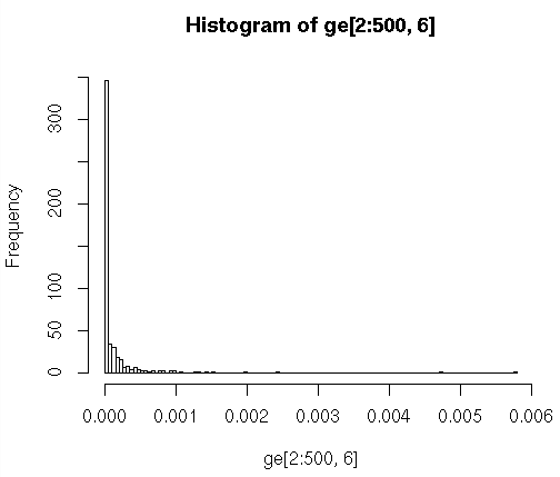
To draw a histogram of a data vector and spline the distribution curve, using the file cybert-allgene.txt (Copy the link location, then wget it to your HPC dir)
In another bash shell (open another terminal session or use byobu)
# take a look at it with 'head'
bash $ head cybert-allgene.txt  # try it, it's not pretty

bash $ cols < cybert-allgene.txt | less -S  # try it, scroll with arrows;

# now switch back to the R session

> bth <- read.table(file=" cybert-allgene.txt",header=TRUE,sep="\t",comment.char="#")

# hmm - why didn't that work?  Oh yes, included an extra leading space.

> bth <- read.table(file="cybert-allgene.txt",header=TRUE,sep="\t",comment.char="#")

# better.  Now check it with the str() function (shows the 'structure' of the object.)

> str(bth)
'data.frame':   500 obs. of  21 variables:
 $ L         : Factor w/ 500 levels "GH01001","GH01027",..: 416 491 67 462 452 409 253 257 191 309 ...
 $ R1        : num  -0.673 NA 0.152 -0.596 1.526 ...
 $ R2        : num  -0.37 -0.7 -0.743 -0.455 -0.238 ...
 $ R3        : num  -0.272 -0.467 -0.833 -0.343 1.413 ...
 $ R4        : num  -1.705 -1.679 -1.167 -0.376 0.362 ...
 $ R5        : num  -0.657 -0.962 -0.376 -0.289 0.698 ...
 $ ExprEst   : num  -0.111 NA -0.0364 0.0229 0.0921 ...
 $ nR        : int  5 4 5 5 5 5 5 5 5 4 ...
 $ meanR     : num  -0.735 -0.952 -0.593 -0.412 0.752 ...
 $ stdR      : num  0.57 0.525 0.503 0.119 0.737 ...
 $ rasdR     : num  0.306 0.491 0.282 0.308 0.425 ...
 $ bayesSD   : num  0.414 0.519 0.373 0.278 0.553 ...
 $ ttest     : num  -3.97 -3.67 -3.56 -3.31 3.04 ...
 $ bayesDF   : int  13 12 13 13 13 13 13 13 13 12 ...
 $ pVal      : num  0.00161 0.00321 0.00349 0.00566 0.00949 ...
 $ cum.ppde.p: num  0.0664 0.1006 0.1055 0.1388 0.1826 ...
 $ ppde.p    : num  0.105 0.156 0.163 0.209 0.266 ...
 $ ROC.x     : num  0.00161 0.00321 0.00349 0.00566 0.00949 ...
 $ ROC.y     : num  0.000559 0.001756 0.002009 0.004458 0.010351 ...
 $ Bonferroni: num  0.805 1 1 1 1 ...
 $ BH        : num  0.581 0.581 0.581 0.681 0.681 ...

# Create a histogram for the 'R2' column.  The following cmd not only plots the histogram
# but also populates the 'hhde' histogram object.
# breaks =  how many bins there should be (controls the size of the bins
# plot = to plot or not to plot
# labels = if T, each bar is labeled with the numeric value
# main, xlab, ylab = plot title, axis labels
# col = color of hist bars
# ylim, xlim = axis limits; if not set, the limits will be those of the data.

> hhde <-hist(bth$R2,breaks=30,plot="True",labels=F, main="Ratio Distribution (R2)",xlab="Ratio",ylab="Frequency", col="lightblue",ylim=c(0,100), xlim=c(-1.7,1.0))

# now plot a smoothed distribution using the hhde$mids (x) and hhde$counts (y)
# df = degrees of freedom, how much smoothing is applied;
#    (how closely the line will follow the values)
> lines(smooth.spline(hhde$mids,hhde$counts, df=20), lty=1, col = "brown")
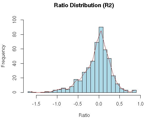
22.10. Basic Statistics
Now (finally) let’s get some basic descriptive stats out of the original table. 1st, load the lib that has the functions we’ll need
> library(pastecs)  # load the lib that has the correct functions

> attach(ge) # make the C1.1 & C1.0 columns usable as variables.

# following line combines an R data structure by column.
# type 'help(cbind)' or '?cbind' for more info on cbind, rbind

> c1all <- cbind(C1.1,C1.0)

# the following calculates a table of descriptive stats for both the C1.1 & C1.0 variables
> stat.desc(c1all)
                      C1.1         C1.0
nbr.val       5.980000e+02 5.980000e+02
nbr.null      3.090000e+02 3.150000e+02
nbr.na        0.000000e+00 0.000000e+00
min          -3.363966e-02 0.000000e+00
max           0.000000e+00 1.832408e-02
range         3.363966e-02 1.832408e-02
sum          -1.787378e-01 8.965868e-02
median        0.000000e+00 0.000000e+00
mean         -2.988927e-04 1.499309e-04
SE.mean       6.688562e-05 3.576294e-05
CI.mean.0.95  1.313597e-04 7.023646e-05
var           2.675265e-06 7.648346e-07
std.dev       1.635624e-03 8.745482e-04
coef.var     -5.472277e+00 5.833009e+00
You can also feed column numbers (as opposed to variable names) to stat.desc to generate similar results:
stat.desc(some_table[2:13])
             stress_ko_n1 stress_ko_n2 stress_ko_n3 stress_wt_n1 stress_wt_n2
nbr.val      3.555700e+04 3.555700e+04 3.555700e+04 3.555700e+04 3.555700e+04
nbr.null     0.000000e+00 0.000000e+00 0.000000e+00 0.000000e+00 0.000000e+00
nbr.na       0.000000e+00 0.000000e+00 0.000000e+00 0.000000e+00 0.000000e+00
min          1.013390e-04 1.041508e-04 1.003806e-04 1.013399e-04 1.014944e-04
max          2.729166e+04 2.704107e+04 2.697153e+04 2.664553e+04 2.650478e+04
range        2.729166e+04 2.704107e+04 2.697153e+04 2.664553e+04 2.650478e+04
sum          3.036592e+07 2.995104e+07 2.977157e+07 3.054361e+07 3.055979e+07
median       2.408813e+02 2.540591e+02 2.377578e+02 2.396799e+02 2.382967e+02
mean         8.540068e+02 8.423388e+02 8.372915e+02 8.590042e+02 8.594593e+02
SE.mean      8.750202e+00 8.608451e+00 8.599943e+00 8.810000e+00 8.711472e+00
CI.mean.0.95 1.715066e+01 1.687283e+01 1.685615e+01 1.726787e+01 1.707475e+01
var          2.722458e+06 2.634967e+06 2.629761e+06 2.759796e+06 2.698411e+06
std.dev      1.649987e+03 1.623258e+03 1.621654e+03 1.661263e+03 1.642684e+03
coef.var     1.932054e+00 1.927085e+00 1.936785e+00 1.933941e+00 1.911300e+00

<etc>
There is also a basic function called summary, which will give summary stats on all components of a dataframe.
> summary(ge)
> summary(ge)
       b                gene            EC           C1.0
 b0001  :  1   0          : 20   0       :279   Min.   :0.000e+00
 b0002  :  1   0.000152968:  1   1.10.3.-:  4   1st Qu.:0.000e+00
 b0003  :  1   0.000158799:  1   2.7.7.7 :  4   Median :0.000e+00
 b0004  :  1   3.32E-06   :  1   5.2.1.8 :  4   Mean   :1.499e-04
 b0005  :  1   3.44E-05   :  1   5.-.-.- :  3   3rd Qu.:7.375e-05
 b0006  :  1   6.66E-05   :  1   1.-.-.- :  2   Max.   :1.832e-02
 (Other):592   (Other)    :573   (Other) :302
      C1.1                 C2.0                C2.1
 Min.   :-0.0336397   Min.   :0.0000000   Min.   :0.000e+00
 1st Qu.:-0.0001710   1st Qu.:0.0000000   1st Qu.:0.000e+00
 Median : 0.0000000   Median :0.0000000   Median :0.000e+00
 Mean   :-0.0002989   Mean   :0.0001423   Mean   :1.423e-04
 3rd Qu.: 0.0000000   3rd Qu.:0.0000754   3rd Qu.:5.927e-05
 Max.   : 0.0000000   Max.   :0.0149861   Max.   :1.462e-02

 [ rest of output trimmed ]
This is only the very beginning of what you can do with R. We’ve not even touched on the Bioconductor suite, which is one of the best known and supported tools to deal with Bioinformatics.
22.11. Visualizing Data with ggobi
While there are many ways in R to plot your data, one unique benefit that R provides is its interface to ggobi, an advanced visualization tool for multivariate data, which for the sake of argument is more than 3 variables.
rggobi takes an R dataframe and presents the variables in a very sophisticated way in realtime 3D, allowing you to visualize multiple variables in multiple ways.
> library("rggobi")  # load the library
> g <- ggobi(ge)     # R dataframe -> a ggobi object, and starts ggobi with that object

# were going to use the 'mtcars' data set which is a bunch of car data.
> g <- ggobi(mtcars)

# Now you have access to the entire ggobi interface via point and click (tho there are still a lot of choices and not all of them are straightforward)
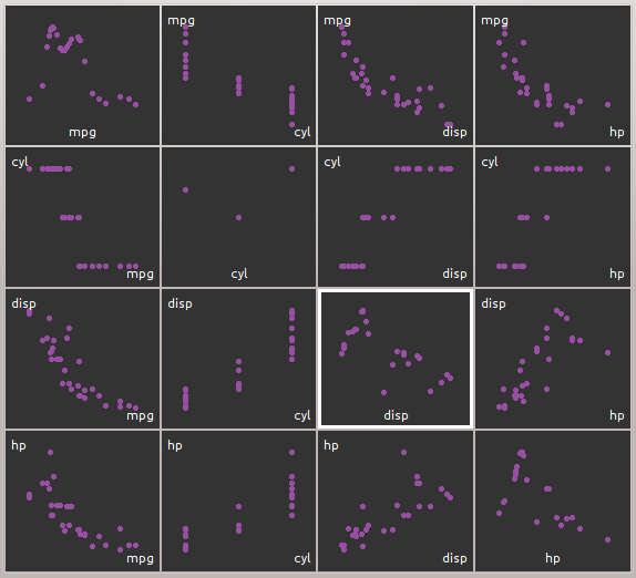
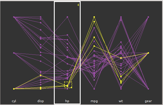
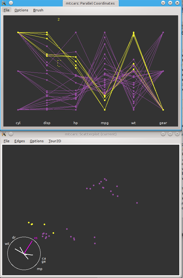
22.12. Using HDF5 files with R
HDF5 (see also the Wikipedia entry) is a very sophisticated format for data which is being used increasingly in domains that were not previously using it, chiefly in Financial Record Archiving, and Bioinformatics.
As the name suggests, internally, it is a hierarchically organized hyperslab, a structure of multi-dimensional arrays of the same data type (ints, floats, bools, etc), sort of like the file equivalent of a C struct. There can be multiple different such arrays but each contains data of the same type.
R supports reading and writing HDF5 files with the rhdf5 library, among others.
22.12.1. Reading HDF5 files into R
You might also look at the HDF5 format section and tutorial below. Using the HDFView java app allows you visualize how the HDF5 file is laid out and enables a pointy-clicky introduction to what the data are. You’ll need to have a Graphics window open, either a true X11 client or preferably x2go.
First, get a small (12MB) HDF5 file:
wget  http://moo.nac.uci.edu/~hjm/biolinux/bigdata/SVM_noaa_ops.h5

# then module load the HDF5 library and apps
module load hdf5/1.8.13

# open hdfview.sh with the just-downloaded file
hdfview.sh SVM_noaa_ops.h5
The HDFView window should open on your screen with the file already loaded. Explore the data structure by opening the groups and arrays and try to visualize them in various ways.
If you are only going to be reading HDF5 files provided by others, the approach is very easy:
# load R
module load R/0_3.1.1

# and start it
R

# assuming the rhdf5 library is installed
> library(rhdf5)
> h5 <- h5read("SVM_noaa_ops.h5")  # a 12MB HDF5 file
> h5ls("SVM_noaa_ops.h5")         # describe the structure of the HDF5 file
                         group                  name       otype    dclass
0                            /              All_Data   H5I_GROUP
1                    /All_Data      VIIRS-M1-SDR_All   H5I_GROUP
2   /All_Data/VIIRS-M1-SDR_All              ModeGran H5I_DATASET   INTEGER
3   /All_Data/VIIRS-M1-SDR_All              ModeScan H5I_DATASET   INTEGER
4   /All_Data/VIIRS-M1-SDR_All  NumberOfBadChecksums H5I_DATASET   INTEGER
5   /All_Data/VIIRS-M1-SDR_All NumberOfDiscardedPkts H5I_DATASET   INTEGER
6   /All_Data/VIIRS-M1-SDR_All   NumberOfMissingPkts H5I_DATASET   INTEGER
7   /All_Data/VIIRS-M1-SDR_All         NumberOfScans H5I_DATASET   INTEGER
8   /All_Data/VIIRS-M1-SDR_All              PadByte1 H5I_DATASET   INTEGER
9   /All_Data/VIIRS-M1-SDR_All     QF1_VIIRSMBANDSDR H5I_DATASET   INTEGER
10  /All_Data/VIIRS-M1-SDR_All          QF2_SCAN_SDR H5I_DATASET   INTEGER
11  /All_Data/VIIRS-M1-SDR_All          QF3_SCAN_RDR H5I_DATASET   INTEGER
12  /All_Data/VIIRS-M1-SDR_All          QF4_SCAN_SDR H5I_DATASET   INTEGER
13  /All_Data/VIIRS-M1-SDR_All  QF5_GRAN_BADDETECTOR H5I_DATASET   INTEGER
14  /All_Data/VIIRS-M1-SDR_All              Radiance H5I_DATASET   INTEGER
15  /All_Data/VIIRS-M1-SDR_All       RadianceFactors H5I_DATASET     FLOAT
16  /All_Data/VIIRS-M1-SDR_All           Reflectance H5I_DATASET   INTEGER
17  /All_Data/VIIRS-M1-SDR_All    ReflectanceFactors H5I_DATASET     FLOAT
18                           /         Data_Products   H5I_GROUP
19              /Data_Products          VIIRS-M1-SDR   H5I_GROUP
20 /Data_Products/VIIRS-M1-SDR     VIIRS-M1-SDR_Aggr H5I_DATASET REFERENCE
21 /Data_Products/VIIRS-M1-SDR   VIIRS-M1-SDR_Gran_0 H5I_DATASET REFERENCE
          dim
0
1
2           1
3          48
4          48
5          48
6          48
7           1
8           3
9  3200 x 768
10         48
11         48
12        768
13         16
14 3200 x 768
15          2
16 3200 x 768
17          2
18
19
20         16
21         16

# in a slightly different format, 'h5dump' provides similar information:
> h5dump(file="SVM_noaa_ops.h5", load=FALSE)
$All_Data
$All_Data$`VIIRS-M1-SDR_All`
$All_Data$`VIIRS-M1-SDR_All`$ModeGran
  group     name       otype  dclass dim
1     / ModeGran H5I_DATASET INTEGER   1

$All_Data$`VIIRS-M1-SDR_All`$ModeScan
  group     name       otype  dclass dim
1     / ModeScan H5I_DATASET INTEGER  48

 ... <etc>
Other R data manipulations are fairly easy as well.
# you can read parts of the HDF5 hyperslab into an R variable as well
# the following reads a subgroup into an R object
> h5_aa <- h5read("SVM_noaa_ops.h5", "/All_Data/VIIRS-M1-SDR_All")

# and this is what h5_aa contains.
> names(h5_aa)
 [1] "ModeGran"              "ModeScan"              "NumberOfBadChecksums"
 [4] "NumberOfDiscardedPkts" "NumberOfMissingPkts"   "NumberOfScans"
 [7] "PadByte1"              "QF1_VIIRSMBANDSDR"     "QF2_SCAN_SDR"
[10] "QF3_SCAN_RDR"          "QF4_SCAN_SDR"          "QF5_GRAN_BADDETECTOR"
[13] "Radiance"              "RadianceFactors"       "Reflectance"
[16] "ReflectanceFactors"

# see each sub-object by referencing it in the standard R way:
> h5_aa$NumberOfScans
[1] 48
22.12.2. Writing HDF5 files from R
Writing HDF5 files is slightly more difficult, but only because you have to be careful that you’re writing to the right group and that there is congruence between R and HDF5 data types and attributes. The rhdf5 docs have good examples for this.
22.13. Exporting Data from R
Ok, you’ve imported your data, analyzed it, generated some nice plots and dataframes. How do you export it to a file so it can be read by other applications? As you might expect, R provides some excellent documentation for this as well. The previously noted document R Data Import/Export describes it well. It’s definitely worthwhile reading it in full, but the very short version is that the most frequently used export function is to write dataframes into tabular files, essentially the reverse of reading Excel spreadsheets, but in text form. For this, we most often use the write.table() function. Using the ge dataframe already created, let’s output some of it:
> ge[1:3,] # lets see what it looks like 'raw'
      b             gene              EC        C1.0         C1.1        C2.0
1 b0001             thrL     0.000423101 0.000465440 -0.000858524 0.000433869
2 b0002 thrA+thrA1+thrA2 1.1.1.3+2.7.2.4 0.001018277 -0.002536156 0.001312524
3 b0003             thrB        2.7.1.39 0.000517967 -0.000915210 0.000582354
         C2.1        C3.0        C3.1        E1.0        E1.1        E2.0
1 0.000250998 0.000268929 0.000369315 0.000736700 0.000712840 0.000638379
2 0.001398845 0.000780489 0.000722073 0.001087711 0.001453382 0.002137451
3 0.000640462 0.000374730 0.000409490 0.000437738 0.000559135 0.000893933
         E2.1        E3.0        E3.1      C1.1Neg
1 0.000475292 0.000477763 0.000509705 -0.000429262
2 0.002153896 0.001605332 0.001626144 -0.001268078
3 0.000839385 0.000621375 0.000638264 -0.000457605


> write.table(ge[1:3,])

"b" "gene" "EC" "C1.0" "C1.1" "C2.0" "C2.1" "C3.0" "C3.1" "E1.0" "E1.1" "E2.0" "E2.1" "E3.0" "E3.1" "C1.1Neg"
"1" "b0001" "thrL" "0.000423101" 0.00046544 -0.000858524 0.000433869 0.000250998 0.000268929 0.000369315 0.0007367 0.00071284 0.000638379 0.000475292 0.000477763 0.000509705 -0.000429262
"2" "b0002" "thrA+thrA1+thrA2" "1.1.1.3+2.7.2.4" 0.001018277 -0.002536156 0.001312524 0.001398845 0.000780489 0.000722073 0.001087711 0.001453382 0.002137451 0.002153896 0.001605332 0.001626144 -0.001268078
"3" "b0003" "thrB" "2.7.1.39" 0.000517967 -0.00091521 0.000582354 0.000640462 0.00037473 0.00040949 0.000437738 0.000559135 0.000893933 0.000839385 0.000621375 0.000638264 -0.000457605

# in the write.table() format above, it's different due to the quoting and spacing.
# You can address all these in the various arguments to write.table(), for example:

> write.table(ge[1:3,], quote = FALSE, sep = "\t",row.names = FALSE,col.names = TRUE)
b       gene    EC      C1.0    C1.1    C2.0    C2.1    C3.0    C3.1    E1.0    E1.1    E2.0  E2.1     E3.0    E3.1    C1.1Neg
b0001   thrL    0.000423101     0.00046544      -0.000858524    0.000433869     0.000250998   0.000268929      0.000369315     0.0007367       0.00071284      0.000638379     0.000475292   0.000477763      0.000509705     -0.000429262
b0002   thrA+thrA1+thrA2        1.1.1.3+2.7.2.4 0.001018277     -0.002536156    0.001312524   0.001398845      0.000780489     0.000722073     0.001087711     0.001453382     0.002137451   0.002153896      0.001605332     0.001626144     -0.001268078
b0003   thrB    2.7.1.39        0.000517967     -0.00091521     0.000582354     0.000640462   0.00037473       0.00040949      0.000437738     0.000559135     0.000893933     0.000839385   0.000621375      0.000638264     -0.000457605


# note that I omitted a file specification to dump the output to the screen.  To send
# the same output to a file, you just have to specify it:

> write.table(ge[1:3,], file="/path/to/the/file.txt", quote = FALSE, sep = "\t",row.names = FALSE,col.names = TRUE)


# play around with the arguments, reversing or modifying the argument values.
# the entire documentation for write.table is available from the commandline with
# '?write.table'
22.14. The commercial Revolution R is free to Academics
Recently a company called Revolution Analytics has started to commercialize R, smoothing off the rough edges, providing a GUI, improving the memory management, speeding up some core routines. If you’re interested in it, you can download it from here.
23. Relational Databases
If the data you have depends on defining or extracting formal relationships, a Relational Database may help you organize and query your data. Such a database requires the creation of a formally structured database, consisting of one or more Tables whose content can be queried via the Structured Query Language (SQL).
The software for doing this are widely available, both proprietary (Oracle, Microsoft) as well as Open Source Software (SQLite, MySQL, PostgreSQL. A great deal of the Internet social media runs on the OSS versions.
For many research problems, you will probably need only a Relational Engine like SQLite, not a full database (which requires both the relational engine as well as the administration, network, user, and security software to make it available over a network. SQLite is the overwhelming relational engine of choice for a single-user relational engine. It’s in a lot of the software you use already - from iTunes to Dropbox to Firefox to to Airbus.
For larger, more distributed problems, you may need the reach and abilities of a full-on Relational Database Management System such as MySQL or PostgreSQL.
For this exercise, we exploit both. First, we can use an Internet-help page that already provides an existing Database with which you can experiment. Go to the surprisingly good the W3Schools start page.
There, you should see a 3-paned window. The top left pane allows entry of arbitrary SQL, ther results of which show up in the lower left pane, while the right pane shows the Database tables.
Click through the Tables to see how they’re laid out and what kind of information they contain. The Customers, Categories, Employees, Products, Shippers and Suppliers are easily human readable and provide the underlying information. OrderDetails and Orders are mostly relational information - they provide the inter-linking information among Tables.
The page on which you first landed already had an SQL query executed:
SELECT * FROM [Products]
and the results shown below. You can now experiment with variants of that SQL query by pasting in the following SQL statements to see how they change the results.
SELECT * FROM [Customers]

SELECT Country  FROM [Customers]

SELECT distinct Country  FROM [Customers]

SELECT distinct city  FROM Customers c where c.Country = "Germany"

SELECT distinct city  FROM Customers c where c.Country = "France"

SELECT City FROM [Customers] where Customers.Country like "Germa%"

# following shows the results of a JOIN operation between Tables
SELECT Orders.OrderID, Customers.CustomerName, Orders.OrderDate
FROM Orders
INNER JOIN Customers
ON Orders.CustomerID=Customers.CustomerID;

#The following shows the results from a UNION operation
SELECT City FROM Customers
UNION
SELECT City FROM Suppliers
ORDER BY City;
There is an entire SQL tutorial available on that website.
24. BigData file formats
|
|
The is a difference between HDFS and HDF5
Despite both being strongly associated with BigData and the acronymic similarity, HDFS (Hadoop File System) and HDF5 (Hierarchical Data Format) are quite different. HDFS is underlying special-purpose filesystem for Apache Hadoop. HDF5 is a file format for storing very large datasets. There is a very good good comparison between them, with the quotable summary line" Think of Hadoop as the single cup coffee maker and HDF5 as one form factor of coffee packs. |
There are a number of BigData file formats that are specialized for storing vast amounts of data, from Astronomy data to Satellite images to Stock Trading logs to Genomic data. Some examples are:
Some of these have been explicitly designed for a particular domain - the Flexible Image Transport System (FITS) format was designed for astronomical image data and isn’t used widely outside of that domain. However, files like the recently converging netCDF and HDF5 formats are general enough that they are now being used across a large number of domains, including bioinformatics, Earth System Science, Financial sectors, etc.
Due to the increasing size of Scientific data, we will be seeing more data supplied in this format, which does seem to be the next-gen version of ASCII data and already many commercial and OSS applications support it either in their base version or via plug-ins or libraries. Such apps include most of the usual suspects:
-
MATLAB (and MATLAB’s default .mat format IS apparently an HDF5 file with a funny header)
-
R, via the rhdf5 library
-
Python / NumPy / SciPy via h5py, (see here for example) Pytables, and ViTables.
-
Perl, via the Perl Data Language and the PDL::IO::HDF5 module.
-
Open Database Connectivity (ODBC) driver that allows an HDF5 file to be opened as a Database to allow import and export to just about any analytical system.
-
SAS - surprisingly, not so much
-
SPSS - surprisingly, not so much
Since the HDF5 format seems to be one of the better-supported BigData formats, we’ll take some time to examine it in more detail.
24.1. HDF5 format
I described how to read HDF5 files using R above, but this section will cover some other aspects of using them, especially how to view the contents in ways that are fairly easy to comprehend.
HDF5 is a hierarchical collection of hyperslabs - essentially a filesystem-like collection of multi-dimensional arrays, each composed of the same data type (like integers, floats, booleans, strings, etc). These array dimensions can be arbitarily extended in one dimension (usually time), and have a number of characteristics that make them attractive to very large sets of data.
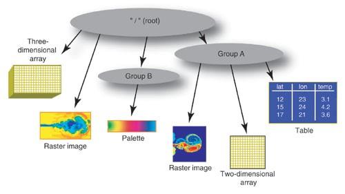
And altho, you can access an HDF5 file sort of like a database (with the ODBC shim, noted above) and PyTables allows doing cross-array queries, it’s definitely NOT a relational data structure. Instead of being used to store relational data, it’s used to store very large amounts of (usually) numeric data that is meant to be consumed in entire arrays (or stripes thereof), analyzed or transformed, and then written back to another HDF5 array.
24.1.1. HDFView tutorial
For the HDF5-naive user, it is difficult to visualize what an HDF5 file looks like or how one is supposed to think about it. Herewith, a demo, one that requires the x2go client.
-
open the x2go client with the gnome terminal
-
If you haven’t already downloaded the test HDF5 file, please do it now.
wget http://moo.nac.uci.edu/~hjm/biolinux/bigdata/SVM_noaa_ops.h5
-
Then load the HDF5 module
module load hdf5/1.8.13
hdfview.sh  #should launch the HDFView java app.
-
Now load the hdf5 file you just downloaded using the File interface
-
And click and double-click your way around them until you have an idea of what the variables and data represent.
-
Note the difference between single value variables, 1 & 2D arrays
-
Try to view the 2D arrays as images
-
Can you plot values?
24.1.2. Python & HDF5 tutorial
Python’s h5py library allows you to access all of the HDF5 API.
As an example of how to read a piece of an HDF5 file from Python, the following scriptlet can print out a 20x20 chunk of a specific Group variable. The problem is that you have to KNOW the the Group Variable name via HDFView or vitables.
# for this example, have to load some modules
module load openmpi-1.6.0/gcc-4.7.3
module load enthought_python/7.3.2

# to visualize the HDF5 internals and get the Variable names.

hdfview.sh  SVM_noaa_ops.h5 &  # works on HPC
# or
vitables    SVM_noaa_ops.h5 &  # may not be installed on HPC.
Following example adapted from here
#!/usr/bin/env python
'''Reads HDF5 file using h5py and prints part of the referenced array'''

import h5py    # HDF5 support

fileName = "SVM_noaa_ops.h5"
f = h5py.File(fileName,  "r")
for item in f.attrs.keys():
    print item + ":", f.attrs[item]

mr = f['/All_Data/VIIRS-M1-SDR_All/QF1_VIIRSMBANDSDR']

for i in range(20):
    print i,
    for j in range(20):
       print mr[i][j],
    print
f.close()
You can download the above code from here (and chmod +x read_hdf5.py) or start up ipython and copy each line in individually to see the result interactively. (in Python, indentation counts.)
24.2. netCDF format
netCDF is another file format for storing complex scientific data. The netCDF factsheet gives a useful overview. In general, netCDF has a simpler structure and at this point, probably more tools available to manipulate the files (esp. nco). netCDF also allows faster extraction of small dataset from large datasets better than HDF5 (which is optimized for complete dataset IO).
Like HDF, there are a variety of netCDF versions, and with each increase in version number, the capabilities increase as well. netCDF is quite similar to HDF in both intent and implementation and the 2 formats are being harmonized into HDF5. A good, brief comparison between the 2 formats is available here. The upshot is that if you are starting a project and have to decide on a format, HDF5 is probably the better choice unless there is a particular advantage of netCDF that you wish to exploit.
However, because there are Exabytes of data in netCDF format, it will survive for decades, and especially if you use climate data and/or satellite data, you’ll probably have to deal with netCDF formats.
25. Resources
25.1. Introduction to Linux
-
The An Introduction to the HPC Computing Facility aka The HPC User’s HOWTO.
-
The BioLinux - a gentle introduction to Bioinformatics on Linux class slides:
-
the topical Biostars StackExchange Resource
-
the SeqAnswer list
-
Instructors:
-
Jenny Wu <jiew5@uci.edu>
-
Harry Mangalam <harry.mangalam@uciedu>
-
If local help is not installed, most R help can be found in PDF and HTML at the R documentation page.
25.2. Local Lightweight Introductions to R
25.3. External Introductions to R
There is a very useful 100 page PDF book called: An Introduction to R (also in HTML). Especially note Chapter 1 and Appendix A on page 78, which is a more sophisticated, (but less gentle) tutorial than this.
Note also that if you have experience in SAS or SPSS, there is a good introduction written especially with this experience in mind. It has been expanded into a large book (to be released imminently), but much of the core is still available for free as R for SAS and SPSS Users
There is another nice Web page that provides a quick, broad intro to R appropriately called Using R for psychological research: A simple guide to an elegant package which manages to compress a great deal of what you need to know about R into about 30 screens of well-cross-linked HTML.
There is also a website that expands on simple tutorials and examples, so after buzzing thru this very simple example, please continue to the QuickR website
Thomas Girke at UC Riverside has a very nice HTML Introduction to R and Bioconductor as part of his Bioinformatics Core, which also runs frequent R-related courses which may be of interest for the Southern California area.
26. Appendix
26.1. Debugging x2go
If you cannot start x2go, check the following:
-
MAKE SURE that the option [ ] Try auto login (ssh-agent or default ssh key) is UNCHECKED if you have not set up ssh keys (and most of you will not have).
-
check the contents of your ~/.x2go dir. It should be empty or nearly so. if it looks like this:
ls ~/.x2go

C-hmangala-324-1392318513_stRgnome-terminal_dp24/  C-hmangala-390-1396546739_stRgnome-terminal_dp24/
C-hmangala-325-1392318654_stRgnome-terminal_dp24/  C-hmangala-50-1394744018_stRgnome-terminal_dp24/
C-hmangala-376-1393961570_stRgnome-terminal_dp24/  C-hmangala-50-1394744071_stRgnome-terminal_dp24/
C-hmangala-383-1395683395_stRxterm_dp24/           C-hmangala-51-1394744050_stRgnome-terminal_dp24/
C-hmangala-384-1395683457_stRxterm_dp24/           C-hmangala-52-1394744202_stRgnome-terminal_dp24/
C-hmangala-385-1395683582_stRxterm_dp24/           C-hmangala-53-1394753487_stRgnome-terminal_dp24/
C-hmangala-386-1395683807_stRgnome-terminal_dp24/  C-hmangala-74-1395682702_stRTerminator_dp24/
C-hmangala-387-1395683950_stRgnome-terminal_dp24/  ssh/
C-hmangala-389-1396546728_stRgnome-terminal_dp24/
then you probably have too many sessions open. Simply delete them all with:
cd ~/.x2go
# make SURE you are in the right dir and then ..
rm -ri *
-
is there a dir called /tmp/.X11-unix on the login host you’re on? It should have permissions like this:
$ ls -ld /tmp/.X11-unix
 drwxrwxrwt 2 root root 4096 Apr  2 19:20 /tmp/.X11-unix/
If it doesn’t exist, please send email to hpc-support@uci.edu telling us that we need to re-create it.
-
make sure the line to the terminal command is spelled correctly. It is:
/usr/bin/gnome-terminal
27. Distribution & Release Conditions
If this Document has been sent to you as a file instead of as a link, some of the content may be lost. The original page is here. The AsciiDoc source is here, which has embedded comments that show how to convert the source to the HTML. AsciiDoc is a simple and simply fantastic documentation language - thanks to Stuart Rackham for developing it.

This work is licensed under a Creative Commons Attribution-ShareAlike 3.0 Unported License.