The latest version of this document will always be found here.
1. Introduction
This tutorial is a follow-on to the previous self-paced tutorial session and extends the basic shell commands described therein to some basic data processing with the Open Source R package.
As such, it assumes that you’re using a Linux system from the bash shell, you’re familiar navigating directories on a Linux system using cd, using the basic shell utilities such as head, tail, less, and grep, and the minimum R system has been installed on your system. If not, you should peruse a basic introduction to the bash shell. The bash prompt in this document is shown as bash $. The R shell prompt is > and R commands will be prefixed by the > to denote it. Inline comments are prefixed by and can be copied into your shell along with the R or bash commands they comment - the shields them from being executed, but do NOT copy in the R or bash shell prompt so mouse carefully.
For a quick introduction to basic data manipulation with Linux, please refer to the imaginatively named Manipulating Data on Linux. It describes in more detail why you might want to know about various Linux text manipulation utilities (to repair data incompatibilities, to scan data sets for forbidden characters, missing values, unexpected negative or positive values - the same things you could do with a spreadsheet and a mouse but MUCH faster.
2. The basic commands in bash
These are the most frequently used general purpose commands that you’ll be using (other than domain-specific applications)
2.1. Logging In, Out, Setting a Display, Moving Around
2.1.1. Local vs Remote
Your laptop is local; HPC is remote. It’e easy to get confused on Linux and a Mac sometimes, especially when executing commands which have a local and remote end, like scp, rsync, and remote displays such as X11, vnc, and x2go.
2.1.2. X11 graphics, vnc, nx, x2go
Linux uses the X11 windowing system to display graphics. As such it needs a program on your local laptop to interpret the X11 data and render them into pixels. All Linux systems come with this already, since it uses X11 as the native display engine. MacOSX also has an X11 display package, now called XQuartz, which has to be started before you can display X11 graphics. Such systems also exist for Windows, but a better alternative for all of them (if you can get it to work) is the x2go system which is more efficient than native X11 (a very chatty protocol and its performance decays rapidly with network hops).
-
Linux: the x2go client seems to work fine, altho the installation will change depending on your distro.
-
MacOSX: the previous version of x2go seems to work fine as long as you start XQuartz 1st.
-
Windows: the latest version seems to work mostly OK. If you need a pure X11 client, try the [free Xming package]. this package proivdes a lot more fonts for the system
2.1.3. Logging In/Out
ssh -Y [UCINETID]@hpc.oit.uci.edu   # getting to HPC
                                    # the '-Y' tunnels the X11 stream thru your ssh connection

exit     # how you exit the login shell
logout   # ditto
^D       # ditto
2.1.4. History & Commandine editing
When you type Enter to execute a command, bash will keep a history of that command. You can re-use that history to recall and edit previous commands
history
history | grep 'obnoxiously long command'
alias hgr="history | grep"
Rather than re-format another page, here is a decent guide to commandline editing in bash. In the very worst case, the arrow keys should work as expected.
2.1.5. Where am I and what’s here?
pwd   # where am I?

# ASIDE: help yourself:  do the following:
# (it makes your prompt useful and tells you where you are)
echo "PS1='\n\t \u@\h:\w\n\! \$ '" >> ~/.bashrc
. ~/.bashrc

ls    # what files are here?  (tab completion)
ls -l
ls -lt
ls -lthS

alias nu="ls -lt |head -20"  # this is a good alias to have

cd       # cd to $HOME
cd -     # cd to dir you were in last (flip/flop cd)
cd ..    # cd up 1 level
cd ../.. # cd up 2 levels
cd dir   # also with tab completion

tree     # view the dir structure pseudo graphically - try it
tree | less  # from your $HOME dir
tree /usr/local |less

mc       # Midnight Commander - pseudo graphical file browser, w/ mouse control

du       # disk usage
du -shc  *

df -h      # disk usage (how soon will I run out of disk)
2.2. Permissions: chmod & chown
Linux has a Unix heritage so everything has an owner and a set of permissions. When you ask for an ls -l listing, the 1st column of data lists the following:
$ ls -l |head
total 14112
-rw-r--r-- 1 hjm hjm   59381 Jun  9  2010 a64-001-5-167.06-08.all.subset
-rw-r--r-- 1 hjm hjm   73054 Jun  9  2010 a64-001-5-167.06-08.np.out
-rw-r--r-- 1 hjm hjm     647 Apr  3  2009 add_bduc_user.sh
-rw-r--r-- 1 hjm hjm    1342 Oct 18  2011 add_new_claw_node
drwxr-xr-x 2 hjm hjm    4096 Jun 11  2010 afterfix/
|-+--+--+-
| |  |  |
| |  |  +-- other permissions
| |  +----- group permissions
| +-------- user permissions
+---------- directory bit

drwxr-xr-x 2 hjm hjm    4096 Jun 11  2010 afterfix/
| |  |  +-- other can r,x
| |  +----- group can r,x
| +-------- user can r,w,x the dir
+---------- it's a directory

# now change the 'mode' of that dir using 'chmod':
chmod -R o-rwx afterfix
         ||-+-
         || |
         || +-- change all attributes
         |+---- (minus) remove the attribute characteristic
         |      can also add (+) attributes, or set them (=)
         +----- other (everyone other than user and explicit group)

$ ls -ld  afterfix
drwxr-x--- 2 hjm hjm 4096 Jun 11  2010 afterfix/

# Play around with the chmod command on a test dir until you understand how it works
chown (change ownership) is more direct; you specifically set the ownership to what you want, altho on HPC, you’ll have limited ability to do this since you can only change your group to to another group of which you’re a member. You can’t change ownership of a file to someone else, unless you’re root.
$ ls -l gromacs_4.5.5.tar.gz
-rw-r--r-- 1 hmangala staff 58449920 Mar 19 15:09 gromacs_4.5.5.tar.gz
                      ^^^^^
$ chown hmangala.stata  gromacs_4.5.5.tar.gz

$ ls -l gromacs_4.5.5.tar.gz
-rw-r--r-- 1 hmangala stata 58449920 Mar 19 15:09 gromacs_4.5.5.tar.gz
                      ^^^^^
2.3. Moving, Editing, Deleting files
These are utilities that create and destroy files and dirs. Deletion on Linux is not warm and fuzzy. It is quick, destructive, and irreversible. It can also be recursive.
|
|
Warning: Don’t joke with a Spartan
Remember the movie 300 about Spartan warriors? Think of Linux utilities like Spartans. Don’t joke around. They don’t have a great sense of humor and they’re trained to obey without question. A Linux system will commit suicide if you ask it to. |
rm  my/thesis            # instantly deletes my/thesis
alias rm="rm -i"         # Please God, don't let me delete my thesis.

# alias logout="echo 'fooled ya'"    can alias the name of an existing utility for anything.
# unalias is the anti-alias.

mkdir dirname            # for creating dirname
rmdir dirname            # for destroying dirname if empty

cp from/here  to/there   # COPIES from/here  to/there
mv  from/here  to/there  # MOVES  from/here  to/there (from/here is deleted!)

file this/file           # what kind of file is this/file?

nano/joe/vi/vim/emacs    # terminal text editors
gedit/nedit/jedit/xemacs # GUI editors
2.4. STDIN STDOUT STDERR: Controlling data flow
These are the input/output channels that Linux provides for communicating among your input, and program input and output
-
STDIN, usually attached to the keyboard. You type, it goes thru STDIN and shows up on STDOUT
-
STDOUT, usually attached to the terminal screen. Shows both your STDIN stream and the program’s STDOUT stream as well as …
-
STDERR, also usually connected to the terminal screen, which as you might guess, sometimes causes problems when both STDOUT and STDERR are both writing to the screen.
wc < a_file     # wc reads a_file on STDIN and counts lines, words, characters

ls -1 > a_file  # ls -1 creates & writes to  'a_file' on STDOUT
ls -1 >> a_file  # ls -1 appends to 'a_file' on STDOUT

someprogram 2> the_stderr_file        # the STDERR creates and writes into 'the_stderr_file'
someprogram &> stdout_stderr_file     # both STDER and STDOUT are captured in 'stdout_stderr_file'

# A real example
module load tacg  # module sets up all the PATHS, etc for tacg

tacg -n6 -slLc -S -F2 < tacg-4.6.0-src/Seqs/hlef.seq | less  # what does this do?
#  vs
tacg -n6 -slLc -S -F2 < tacg-4.6.0-src/Seqs/hlef.seq > less  # what does this do?

tacg -n6 -slLc -S -F2 < tacg-4.6.0-src/Seqs/hlef.seq > out   # what does this do?
2.4.1. Pipes
You can redirect all these channels via various currently incomprehensible incantations, but this is a really important concept, explained in more detail here. A program’s STDOUT output can be connected to another program’s STDIN input via a pipe which is represented in Linux as | (vertical bar).
For example:
ls -1    # prints all the files in the current dir 1 line at a time
wc       # counts the lines, words, characters passed to it via STDIN

ls -1 | wc  # the number of lines, etc that 'ls -1' provides, or the # of files in the dir
This is a powerful concept in Linux that doesn’t have a good parallel in Windows.
2.5. Viewing & Slicing Data
2.5.1. Pagers, head & tail
less & more are pagers, used to view text files. In my opinion, less is better than more, but both will do the trick.
less somefile  # try it

alias less='less -NS' # is a good setup (number lines, scroll for wide lines)


head -###  file2view  # head views the top ### lines of a file, tail views the bottom
tail -###  file2view  # tail views the ### bottom lines of a file
tail -f    file2view  # keeps dumping the end of the file if it's being written to.
2.5.2. Concatenating files
Sometimes you need to concatenate / aggregate files; for this, cat is the cat’s meow.
cat file2view                    # dumps it to STDOUT
cat file1 file2 file3 > file123  # or concatenates multiple files to STDOUT, captured by '>' into file123
2.5.3. Slicing out columns, rectangular selections
cut and scut allow you to slice out columns of data by acting on the tokens by which they’re separated. A token is just the delimiter between the columns, typically a space or <tab>, but it could be anything, even a regex. cut only allows single characters as tokens, scut allows any regex as a token.
cut -f# -d[delim char]                 # cuts out the fth field (counts from 1)
scut -f='2 8 5 2 6 2'  -d='pcre delim' # cuts out whatever fields you want;
#  allows renumbering, repeating, with a 'perl compatible regular expression' delimiter
Use cols to view data aligned to columns.
cols < MS21_Native.txt | less   # aligns the top lines of a file to view in columns
#  compare with
less  MS21_Native.txt
Many editors allow columnar selections and for small selections this may be the best approach Linux editors that support rectangular selection
| Editor | Rectangular Select Activation |
|---|---|
nedit |
Ctrl+Lmouse = column select |
jedit |
Ctrl+Lmouse = column select |
kate |
Shift+Ctrl+B = block mode, have to repeat to leave block mode. |
emacs |
dunno - emacs is more a lifestyle than an editor but it can be done. |
vim |
Ctrl+v puts you into visual selection mode. |
2.5.4. Finding file differences and verifying identity
Quite often you’re interested the differences between 2 related files or verifying that the file you sent is the same one as arrived. diff and especially the GUI wrappers (diffuse, kompare) can tell you instantly.
diff file1 file1a          # shows differences between file1 and file2
diff hlef.seq hlefa.seq      # on hpc


md5sum files           # lists MD5 hashes for the files
# md5sum is generally used to verify that files are identical after a transfer.
# md5 on MacOSX, <http://goo.gl/yCIzR> for Windows.
2.6. The grep family
Sounds like something blobby and unpleasant and sort of is, but it’s VERY powerful. Regular Expressions are formalized patterns. As such they are not exactly easy to read at first, but it gets easier with time.
The simplest form is called globbing and is used within bash to select files that match a particular pattern
ls -l *.pl    # all files that end in '.pl'
ls -l b*.     # all files that start with 'b' & end in '.pl'
ls -l b*p*.*l  # all files that start with 'b' & have a 'p' & end in 'l'
Looking at nucleic acids, can we encode this into a regex?:
gyrttnnnnnnngctww = g[ct][ag]tt[acgt]{7}gct[at][at]
grep regex files   # look for a regular expression in these files.
grep -rin regex  *  # recursively look for this case-INsensitive regex in all files and
                    # dirs from here down to the end and number the lines.
grep -v regex files # invert search (everything EXCEPT this regex)
egrep "thisregex|thatregex" files  # search for 'thisregex' OR 'thatregex' in these files

egrep "AGGCATCG|GGTTTGTA" hlef.seq

# gnome-terminal allows searching in output, but not as well as 'konsole'
2.7. Getting Data to and from HPC
scp paths/to/sources/*  user@host:/path/to/target       # always works on Linux/MacOSX
scp ~/nacs/nco-4.2.5.tar.gz  hmangala@hpc.oit.uci.edu:~

wget URL     # drops file in current dir
wget http://hpc.oit.uci.edu/biolinux/data/tutorial_data/hlef.seq

curl URL     # spits out file to STDOUT
curl http://hpc.oit.uci.edu/biolinux/data/tutorial_data/hlef.seq  # ugh...
curl -O http://hpc.oit.uci.edu/biolinux/data/tutorial_data/hlef.seq  # better

#  What does this do then?
curl http://hpc.oit.uci.edu/biolinux/data/tutorial_data/numpy-1.6.1.tar.gz | tar -xzvf -

# rsync 'syncs' files between 2 places by only transferring the bits that have changed.
# (there is also a GUI version of rsync called grsync on HPC.

# the following will not work for you (I hope) since you don't have my passwords
# modify it to try an rsync to your Mac or to another directory on HPC.

rsync -avz nco-4.2.5  hjm@moo:~/backups/hpc/nco-4.2.5
echo "dfh lkhslkhf" >>  nco-4.2.5/configure
rsync -avz nco-4.2.5  hjm@moo:~/backups/hpc/nco-4.2.5  # what's the difference?
2.7.1. tar and zip archives
tar -czvf tarfile.gz files2archive   # create a compressed 'tarball'
tar -tzvf tarfile.gz                 # list the files in a compressed 'tarball'
tar -xzvf tarfile.gz                 # extract a compressed 'tarball'
tar -xzvf tarfile.gz  included/file  # extract a specific 'included/file' from the archive.

# Also, archivemount to manipulate files while still in an archive

# zip is similar, but has a slightly different syntax:

zip zipfilename files2archive        # zip the 'files2archive' into the 'zipfilename'
unzip -l zipfilename.zip             # list the files that are in zipfilename.zip without unzipping them
unzip  zipfilename.zip               # unzip the 'zipfilename.zip' archive into the current dir.
2.8. Info about & Controlling your jobs
top      # lists which are the top CPU-consuming jobs on the node

ps       # lists all the jobs which match the options
ps aux   # all jobs
ps aux | grep hmangala  # all jobs owned by hmangala

alias psg="ps aux | grep"

kill -9 JobPID#   # kill off your job by PID
2.9. Your terminal sessions
You may be spending a lot of time in the terminal session and sometimes the terminal just screws up. If so, you can try typing clear or reset which should reset it.
You will often find yourself wanting multiple terminals to hpc. You can usually open multiple tabs on your terminal but you can also use the byobu app to multiplex your terminal inside of one terminal window. Good help page on byobu here.
The added advantage of using byobu is that the terminal sessions that you open will stay active after you detach from them (usually by hitting F6). This allows you to maintain sessions across logins, such as when you have to sleep your laptop to go home. When you start byobu again at HPC, your sessions will be exactly as you left them.
|
|
A byobu shell in not quite the same as using a direct terminal connection
Because byobu invokes some deep magic to set up the multiple screens, X11 graphics invoked from a byobu-mediated window will sometimes not work, depending on how many levels of shell you’ve descended. Similarly, byobu traps mouse actions so things that might work in a direct connection (mouse control of mc) will not work in a byobu shell. Also some line characters will not format properly. Always tradeoffs… |
2.10. Background and Forground
Your jobs can run in the foreground attached to your terminal, or detached in the background, or simply stopped.
Deep breath…..
-
a job runs in the foreground unless sent to the background with & when started.
-
a foreground job can be stopped with Ctrl+z (think zap or zombie)
-
a stopped job can be started again with fg
-
a stopped job can be sent to the background with bg
-
a background job can be brought to the foregound with fg
If you were going to run a job that takes a long time to run, you could run it in the background with this command.
tar -czf gluster-sw.tar.gz gluster-sw  &   # This would run the job in the background immediately
...
[1]+  Done                    tar -czvf gluster-sw.tar.gz gluster-sw

tar -czvf gluster-sw.tar.gz gluster-sw &  #  Why would this command be sub-optimal?
HOWEVER, for most long-running jobs, you will be submitting the jobs to the scheduler to run in batch mode. See here for how to set up a qsub run.
2.11. Finding files with find and locate
Even the most organized among you will occasionally lose track of where your files are. You can generally find them on HPC by using the find command:
# choose the nearest dir you remember the file might be and then direct find to use that starting point
find [startingpoint] -name filename_pattern

# ie:  (you can use globs but they have to be 'escaped' with a '\'
find gluster-sw/src -name config\*
gluster-sw/src/glusterfs-3.3.0/argp-standalone/config.h
gluster-sw/src/glusterfs-3.3.0/argp-standalone/config.h.in
gluster-sw/src/glusterfs-3.3.0/argp-standalone/config.log
gluster-sw/src/glusterfs-3.3.0/argp-standalone/config.status
gluster-sw/src/glusterfs-3.3.0/argp-standalone/configure
gluster-sw/src/glusterfs-3.3.0/argp-standalone/configure.ac
gluster-sw/src/glusterfs-3.3.0/xlators/features/marker/utils/syncdaemon/configinterface.py


# 'locate' will work on system files, but not on user files. Useful for looking for libraries,
# but probably not in the module files

locate libxml2 |head   # try this

# Also useful for searching for libs is 'ldconfig -v', which searches thru the LD_LIBRARY_PATH

ldconfig -v |grep libxml2
2.12. Modules
Modules are how we maintain lots of different applications with mutiple versions without (much) confusion. In order to load a particular module, you have to call it up (with the specific version if you don’t want the latest one).
module load app/version  # load the module
module whatis app        # what does it do?
module rm app            # remove this module (doesn't delete the module, just removes the paths to it)
module purge             # removes ALL modules loaded (provides you with a pristine environment)
3. VERY simple bash programming
These code examples do not use the bash $ prefix since they’re essentially stand-alone. The bash commands that are interspersed with the R commands later are so prefixed.
3.1. bash variables
Remember variables from math? A variable is a symbol that can hold the value of something else. In most computer languages (including bash) a variable can contain:
-
numeric values (156, 83773.34 3.5e12, -2533)
-
strings ("booger", "nutcase", "24.334", "and even this phrase")
-
lists or arrays ([12 25 64 98735 72], [238.45 672.6645 0.443 -51.002] or ["if" "you" "have" "to" "ask" "then" "maybe" "…"].
Note that in lists or arrays, the values usually are of the same type (integers, floats, strings, etc). Most languages also allow the use of more highly complex data types (often referred to as data structures, objects, dataframes, etc). Even bash allows you to do this, but it’s so ugly that you’d be better off gouging out your own eyeballs. Use one of Perl, Python, R, Java, etc.
All computer languages allow comments. Often (bash, perl, python, R) the comment indicator is a # which means that anything after the # is ignored.
thisvar="peanut"    # note the spacing
thisvar = "peanut"  # what happened?  In bash, spacing/whitespace matter

thatvar="butter"

echo thisvar

# ?? what happened? Now..

echo $thisvar  # what's the difference?

# note that in some cases, you'll have to protect the variable name with {}

echo $somevar_$thatvar      # what's the difference between this

echo ${somevar}_${thatvar}  # and this?
You can use variables to present the results of system commands if they’re inside of parens ()
seq 1 5  $ what does this do?

filecount=$(seq 1 5)
echo $filecount  # what's the difference in output?


dirlist=$(ls -1)
echo $dirlist
3.2. Looping with bash
Simple bash loops are very useful
for file in *.txt; do
   grep noodle $file
done
3.3. Iterating with loops
for outer in $(seq 1 5); do
  for inner in  $(seq 1 2); do
    # try this with and without variable protection
    echo "processing file bubba_${inner}_${outer}"
  done
done
Can also use this to creat formatted numbers (with leading 0’s)
for outer in $(seq -f "%03g" 1 5); do
  for inner in  $(seq -f "%02g" 1 2); do
    # try this with and without variable protection
    echo "processing file bubba_${inner}_${outer}"
  done
done
There are 1000’s of pages of bash help available. Here’s a good one.
For very simple actions and iterations, especially for apply a set of commands to a set of files, bash is very helpful. For more complicated programmatic actions, I strongly advise using Perl or Python.
4. Simple qsub scripts
For all jobs that take more than a few seconds to run, you’ll be submitting them to the Grid Engine Scheduler. In order to do that, you have to write a short bash script that describes what resources your job will need, how you want your job to produce output, how you want to be notified, what modules your job will need, and perhaps some data staging instructions. Really not hard. Note that in qsub scripts, the GE directives are protected by $. The 1st means that as far as bash is concerned, they’re comments and thus ignored. It’s only GE that will pay attention to the directives behind #$.
Note that using bash variables can make your scripts much more reliable, readable, and maintainable.
A qsub script consists of 4 parts:
-
the shebang line, the name of the shell that will execute the script (almost always #!/bin/bash)
-
comments, prefixed with # that inserted to document what your script does (to both yourself and to us, if you ask for help)
-
the GE directives, prefixed by #$ which set up various conditions and requirements for your job with the scheduler
-
the bash commands that actually describe what needs to be done
#!/bin/bash

# which Q to use?
#$ -q _______

# the qstat job name
#$ -N SLEEPER_1

# use the real bash shell
#$ -S /bin/bash

# mail me ...
#$ -M hmangala@uci.edu

# ... when the job (b)egins, (e)nds
#$ -m be

echo "Job begins"
date

sleep 30

date
echo "Job ends"
#!/bin/bash

# specify the Q run in
#$ -q asom

# the qstat job name
#$ -N RedPstFl

# use the real bash shell
#$ -S /bin/bash

# execute the job out of the current dir and direct the error
# (.e) and output (.o) to the same directory ...
#$ -cwd

# ... Except, in this case, merge the output (.o) and error (.e) into one file
# If you're submitting LOTS of jobs, this halves the filecount and also allows
# you to see what error came at what point in the job.  Recommended unless there's
# good reason NOT to use it.
#$ -j y

#!! NB: that the .e and .o files noted above are the STDERR and STDOUT, not necessarily
#!! the programmatic output that you might be expecting.  That output may well be sent to
#!! other files, depending on how the app was written.

# mail me (hmangala@uci.edu)
#$ -M hmangala@uci.edu

# when the job (b)egins, (e)nds, (a)borts, or (s)uspends
#$ -m beas

############## here

#!! Now note that the commands are bash commands - no more hiding them behind '#$'

# set an output dir in ONE place on the LOCAL /scratch filesystem (data doesn't cross the network)
# note - no spaces before or after the '='
OUTDIR=/scratch/hmangala

# set an input directory.
INDIR=/som/hmangala/guppy_analysis/2.3.44/broad/2013/12/46.599

# and final results dir in one place
FINALDIR=/som/hmangala/guppy/r03-20-2013

MD5SUMDIR=${HOME}/md5sums/guppy/r03-20-2013/md5sums

# make output dirs in the local /scratch and in data filesystem
# I assume that the INDIR already exists with the data in it.
mkdir -p $OUTDIR $FINALDIR

# load the required module
module load guppy/2.3.44

# and execute this command
guppy --input=${INDIR}/input_file --outdir=${OUTDIR} -topo=flat --tree --color=off --density=sparse

# get a datestamp
DATESTAMP=`date|tr /\ / /_/`

# generate md5 checksums of all output data to be able to
# check for corruption if anything happens to the filesystem, god forbid.
md5deep -r $OUTDIR > ${MD5SUMDIR}/md5sums


# copy the md5sums to the output dir to include it in the archive
cp ${MD5SUMDIR}/md5sums ${FINALDIR}


# mail the md5sums to yourself for safekeeping
cat ${MD5SUMDIR}/md5sums | mail -s 'md5sums from HPC' hmangala@uci.edu


# after it finishes, tar up all the data
tar -czf ${FINALDIR}/${DATESTAMP}.tar.gz ${OUTDIR}

# and THIS IS IMPORTANT!! Clean up behind you.
rm -rf $OUTDIR
5. A few seconds with Perl
We’re going to be stepping thru a simple Perl script below, but in order to make it even simpler, here is the core of the program, and it tends to be the core of a huge number of Perl scripts.
But 1st, a word about words .. and delimiters or tokens.
The rain in Spain falls mainly on the plain.\n
0   1    2  3     4     5      6  7   8
Similarly:
-rw-r--r-- 1 root root     69708 Mar 13 22:02 ,1
-rw-r--r-- 1 root root     69708 Mar 13 22:02 ,2
drwxr-xr-x 2 root root      4096 Feb  5 17:07 3ware
-rw------- 1 root root    171756 Dec 13 18:15 anaconda-ks.cfg
-rw-r--r-- 1 root root       417 Feb 22 15:38 bigburp.pl
drwxr-xr-x 2 root root      4096 Mar 26 14:27 bin
drwxr-xr-x 6 root root      4096 Mar 22 15:08 build
-rw-r--r-- 1 root root       216 Feb 22 15:38 burp.pl
drwxr-xr-x 6 root root      4096 Mar 26 15:07 cf
0          1 2    3       4      5   6  7     8
The above outputs all have 8 text fields and CAN be separated on spaces (' '). But what happens in the case below?
-rw-r--r-- 1 root root       216 Feb 22 15:38 burp.pl\n
          _ _    _    _______   _   _  _     _
Breaking on spaces will result not in 8 fields but in 14. Breaking on whitespace will result in 8 fields.
And in this one?
The rain in Spain falls mainly on the plain.\n
Note the leading space? that counts as well.
#!/usr/bin/perl -w
while (<>) {  # while there's still STDIN, read it line by line
#       $N is the # of fields; @A is the array that gets populated
        $N = @A = split(/splitter/, $what_to_split);
        # do something with the @A array and generate $something_useful
        print "$something_useful\n";
}
# from your account on HPC

wget http://moo.nac.uci.edu/~hjm/biolinux/justright.pl

chmod +x justright.pl

# and execute it as below:

ls -l /usr/bin | ./justright.pl 12121 131313

# what does it do?  Let's break it down.. The first part is..

ls -l /usr/bin | cols -d='\s+' | less  # what does this do?

Change the input parameters and try it again to see if you can tell
Well, we have the source code below, so we don’t have to guess. Feel free to open it in an editor, modify it, and try it again.
#!/usr/bin/perl -w
$min = shift;    # assigns 1st param (12121) to $min
$max = shift;    # assigns 2nd param (131313) to $max
while (<>){      # consumes each line in turn and processes it below
        chomp;       # removes the trailing newline (\n)
        @A = split(/\s+/, $_);       # splits $_ on whitespace and loads each el into an array named A
        if ($A[4] < $min) {     # if $A[4] is too small...
                print "ERR: too small ($A[4]):\t[$A[8]]\n";  # print an error
        } elsif ($A[4] > $max) { # if it's too big...
                print "ERR: too big ($A[4]):\t[$A[8]]\n";    # print an error
        } else {
                print "INFO: just right:\t[$A[8]]\n";        # it's just right
                print "$_\n\n";                                # so print the whole line
        }
}
There are 1000’s of pages of Perl help available. Here’s a good one.
6. The R Language
R is a programming language designed specifically for statistical computation. As such, it has many of the characteristics of a general-purpose language including iterators, control loops, network and database operations, many of which are useful, but in general not as easy to use as the more general Python or Perl.
R can operate in 2 modes:
-
as an interactive interpreter (the R shell, much like the bash shell), in which you start the shell and type interactive commands. This is what we’ll be using today.
-
as a scripting language, much like Perl or Python is used, where you assemble serial commands and have the R interpreter run them in a script. Many of the bioinformatics applications writ in R have this form.
Typically the R shell is used to try things out and the serial commands saved in a file are used to automate operations once the sequence of commands is well-defined and debugged. In approach, this is very similar to how we use the bash shell.
7. R is Object Oriented
While R is not a great language for procedural programming, it does excel at mathematical and statistical manipulations. However, it does so in an odd way, especially for those who have done procedural programming before. R is quite object-oriented (OO) in that you tend to deal with data objects rather than with individual integers, floats, arrays, etc. The best way to think of R data if you have programmed in C is to think of R data (typically termed tables or frames) as C structs, arbitrary and often quite complicated structures that can be dealt with by name. If you haven’t programmed in a procedural language, it may actually be easier for you because R manipulates chunks of data similar to how you might think of them. For example, multiply column 17 by 3.54 or pivot that spreadsheet.
The naming system for R’s data objects is similar to other OO naming systems. The sub-object is defined by the name after a "." So a complex data structure named hsgenome might have sub-objects named chr1, chr2, etc, and each of these would have a length associated with it. For example hsgenome.chr1.length might equal 250,837,348, while hsgenome.chr1.geneid341.exon2.length might equal 4347. Obvious, no?
For a still-brief but more complete overview of R’s history, see Wikipedia’s entry for R.
8. Available Interfaces for R
R was developed as a commandline language. However, it has gained progressively more graphics capabilities and graphical user interfaces (GUIs). Some notable examples:
-
the once de facto standard R GUI R Commander,
-
the fully graphical statistics package gretl which was developed external to R for time-series econometrics but which now supports R as an external module
-
Eclipse/StatET, an Eclipse-based Integrated Development Environment (IDE)
-
Rstudio, probably the most advanced R GUI, another full IDE, already available on HPC
-
the extremely powerful interactive graphics utility ggobi, which is not an IDE, but a GUI for multivariate analysis and data exploration.
As opposed to fully integrated commercial applications which have a cohesive and coherent interface, these packages differ slightly in the way that they approach getting things done, but in general the mechanisms follow generally accepted user interface conventions.
In addition, many routines in R are packaged with their own GUIs so that when called from the commandline interface, the GUI will pop up and allow the user to interact with a mouse rather than the keyboard. The extrmely powerful interactive graphics utility ggobi is such a GUI for multivariate analysis and data exploration.
9. Getting help on R
As noted below, when you start R, the 1st screen will tell you how to get local help.
|
|
Don’t copy in the prompt string
Don’t forget that the listed prompts bash $ for bash and > for R are NOT meant to be copied into the shell. ie if the the line reads: bash $ R # more comments on R's startup state below you copy in R. You can copy in the comment line as well (the stuff after the #). It will be ignored by bash, Perl, and R. |
bash $  R  # more comments on R's startup state below

# most startup text deleted ...

Type 'demo()' for some demos, 'help()' for on-line help, or
'help.start()' for an HTML browser interface to help.
Type 'q()' to quit R.

> help.start().
So right away, there’s some useful things to try. By all means try out the demo(). it shows you what R can do, even if you don’t know exactly what how to do it.
And the help.start() will attempt to launch a browser page (from the machine on which R is running, HPC in the case of this tutorial) with a lot of links to R documentation, both introductory and advanced.
See the Resources section at the bottom for many more links to R-related information.
10. Some basic R data types
Before we get too far, note that R has a variety of data structures that may be required for different functions.
Some of the main ones are:
-
numeric - (aka double) the default double-precision (64bit) float representation for a number.
-
integer - a single-precision (32bit) integer.
-
single - a single precision (32bit) float
-
string - any character string ("harry", "r824_09_hust", "888764"). Note the last is a number defined as a string so you couldn’t add "888764" (a string) + 765 (an integer).
-
vector - a series of data types of the same type. (3, 5, 6, 2, 15) is a vector of integers. ("have", "third", "start", "grep) is a vector of strings.
-
matrix - an array of identical data types - all numerics, all strings, all booleans, etc.
-
data.frame - a table (another name for it) or array of mixed data types. A column of strings, a column of integers, a column of booleans, 3 columns of numerics.
-
list - a concatenated series of data objects.
11. Starting R (finally)
We have several versions of R on the HPC cluster, but unless you want to start an older version (in which case you have to specify the version), just type:
bash $ module load R

#    if you then wanted to start Rstudio (and you had set up the necessary graphics options)
#    you would then type:

bash $ rstudio &

#    or if you want the commandline R

bash $ R   #    dumps version info, how to get help, and finally the R prompt

R version 2.15.2 (2012-10-26) -- "Trick or Treat"
Copyright (C) 2012 The R Foundation for Statistical Computing
ISBN 3-900051-07-0
Platform: x86_64-unknown-linux-gnu (64-bit)

R is free software and comes with ABSOLUTELY NO WARRANTY.
You are welcome to redistribute it under certain conditions.
Type 'license()' or 'licence()' for distribution details.

  Natural language support but running in an English locale

R is a collaborative project with many contributors.
Type 'contributors()' for more information and
'citation()' on how to cite R or R packages in publications.

Type 'demo()' for some demos, 'help()' for on-line help, or
'help.start()' for an HTML browser interface to help.
Type 'q()' to quit R.

>
12. Some features of the R interpreter
R supports commandline editing in exactly the same way as the bash shell does. Arrow keys work, command history works, etc.
There is a very nice feature when you try to exit from R that will offer to save the entire environment for you so it can be recreated the next time you log in. If you’re dealing with fairly small data sets (up to a couple hundred MB), it’s very handy sometimes to save the environment. If you’re dealing with a variable set of tens or hundreds of GB, it may not be worth it to try to save the environment, since all that data has to be saved to disk somewhere, duplicating the data in your input files, and also it has to be read back in on restart which may take just about as long as reading in the original files.
The key in the latter (huge data) case is to keep careful records of the commands that worked to transition from one stage of data to another.
If you get the line shown below:
[Previously saved workspace restored]
it indicates that you had saved the previous data environment and if you type ls() you’ll see all the previously created variables:
> ls()
 [1] "ge"          "data.matrix" "fil_ss"      "i"           "ma5"
 [6] "mn"          "mn_tss"      "norm.data"   "sg5"         "ss"
[11] "ss_mn"       "sss"         "tss"         "t_ss"        "tss_mn"
[16] "x"
If the previous session was not saved, there will be no saved variables in the environment
> ls()
character(0) # denotes an empty character (= nothing there)
OK, now let’s quit out of R and NOT save the environment
> quit()
Save workspace image? [y/n/c]: n
13. Loading data into R
Let’s get some data to load into R. Download this file
OK. Got it? Take a look thru it with less
bash $ less GE_C+E.data

#              Notice how the columns don't line up?  Try it again with cols

bash $ cols GE_C+E.data |less

# Notice that the columns now line up?
Loading data into R is described in much more detail in the document R Data Import/Export, but the following will give you a short example of one of the more popular ways of loading data into R.
The following reads the example data file above (GE_C+E.data) into an R table called ge; note the ,header=TRUE option which uses the file header line to name the columns. In order for this to work, the column headers have to be separated by the same delimiter as the data (usually a space or a tab).
> ge <- read.table(file="GE_C+E.data",header=TRUE) # try it
In R, you can work left to right or right to left, altho the left pointing arrow is the usual syntax. The above command could also have been given as :
> read.table(file="GE_C+E.dat",header=TRUE) -> ge # try it
|
|
Problems with reading in a file with read.table
I have run into situations where read.table() would simply not read in a file which I had validated with an external Perl script: ie: > tmp <- read.table(file="long_complicated_data_file",header=TRUE,sep="\t",comment.char="#") Error in scan(file, what, nmax, sep, dec, quote, skip, nlines, na.strings, : line 134 did not have 29 elements In these cases, using read.delim() may be more successful: > em <- read.delim(file="long_complicated_data_file",na.strings = "", fill=TRUE, header=T, sep="\t") (see also Thomas Girke’s excellent R/BioC Guide.) |
OK - did we get the col names labeled correctly?
> names(ge)  # try it
[1] "b"    "gene" "EC"   "C1.0" "C1.1" "C2.0" "C2.1" "C3.0" "C3.1" "E1.0"
[11] "E1.1" "E2.0" "E2.1" "E3.0" "E3.1"
Looks like we did.
Many functions will require the data as a matrix (a data structure whose components are identical data types, usually strings (remember the R data types above? The following will load the same file into a matrix, doing the conversions along the way. This command also shows the use of the sep="\t" option which explicitly sets the data delimiter to the TAB character, as well as how command nesting works in R.
gem <- as.matrix(read.table("GE_C+E.data", sep="\t", header=TRUE))
14. Viewing data
To view some of the table, we only need to reference it. R assumes that a naked variable is a request to view it. An R table is referenced in [rows,column] order. That is, the index is [row indices, col indices], so that a reference like ge[1:6,1:5] will show a square window of the table; rows 1-6, columns 1-5
Let’s try this with the 2 objects we’ve created this far, ge and gem.
# 1st ge, which is a table (can have different data types in it
> ge[1:4,1:5]
      b             gene              EC        C1.0        C1.1
1 b0001             thrL     0.000423101 0.000465440 0.000429262
2 b0002 thrA+thrA1+thrA2 1.1.1.3+2.7.2.4 0.001018277 0.001268078
3 b0003             thrB        2.7.1.39 0.000517967 0.000457605
4 b0004             thrC        4.2.99.2 0.000670075 0.000558063

# now gem which is the same data but as.matrix
> gem[1:4,1:5]
     b       gene               EC                C1.0          C1.1
[1,] "b0001" "thrL"             "0.000423101"     "0.000465440" "0.000429262"
[2,] "b0002" "thrA+thrA1+thrA2" "1.1.1.3+2.7.2.4" "0.001018277" "0.001268078"
[3,] "b0003" "thrB"             "2.7.1.39"        "0.000517967" "0.000457605"
[4,] "b0004" "thrC"             "4.2.99.2"        "0.000670075" "0.000558063"
The 2 data dumps above look similar but are not. gem variables (except for the headers) have all been converted to quoted strings.
Also: R parameters are 1-indexed, not 0-indexed, tho it seems pretty forgiving (if you ask for [0-6,0-5], R will assume you meant [1-6,1-5]. also note that R requires acknowledging that the data structures are n-dimensional: to see rows 1-11, you can’t just type:
> ge[1:11] # try it!
but must instead type:
> ge[1:3,]  # another dimension implied by the ','
      b             gene              EC        C1.0        C1.1        C2.0 <- header
1 b0001             thrL     0.000423101 0.000465440 0.000429262 0.000433869
2 b0002 thrA+thrA1+thrA2 1.1.1.3+2.7.2.4 0.001018277 0.001268078 0.001312524
3 b0003             thrB        2.7.1.39 0.000517967 0.000457605 0.000582354
         C2.1        C3.0        C3.1        E1.0        E1.1        E2.0    <- header
1 0.000250998 0.000268929 0.000369315 0.000736700 0.000712840 0.000638379
2 0.001398845 0.000780489 0.000722073 0.001087711 0.001453382 0.002137451
3 0.000640462 0.000374730 0.000409490 0.000437738 0.000559135 0.000893933
         E2.1        E3.0        E3.1                                        <- header
1 0.000475292 0.000477763 0.000509705
2 0.002153896 0.001605332 0.001626144
3 0.000839385 0.000621375 0.000638264
If the data is too long for a single screen, R will split it up over multiple stanzas, repeating the headers which is nice for viewing.
To slice the table even further, you can view only those elements that interest you
  # R will provide row and column headers if they were provided.
  # if they weren't provided, it will provide column indices.
> ge[3:7,4:5]   # try it.
         C1.0        C1.1
3 0.000517967 0.000457605
4 0.000670075 0.000558063
5 0.000000000 0.000000264
6 0.000000000 0.000000000
7 0.000008870 0.000015400
15. Operations on Data
To operate on a column, ie: to multiply it by some value, you only need to reference the column ID, not each element. This is a key idea behind R’s object-oriented approach. The following multiplies the column C1.1 of the table ge by -1 and stores the result in the column 'C1.1Neg. There’s no need to pre-define the C1.1Neg column; R will allocate space for it as needed.
> ge$C1.1Neg = ge$C1.1 * -1   # try it


# the table now has a new column appended to the end called 'C1.1Neg'
> ge[1:2,]      # try it
      b             gene              EC        C1.0        C1.1        C2.0
1 b0001             thrL     0.000423101 0.000465440 0.000429262 0.000433869
2 b0002 thrA+thrA1+thrA2 1.1.1.3+2.7.2.4 0.001018277 0.001268078 0.001312524
         C2.1        C3.0        C3.1        E1.0        E1.1        E2.0
1 0.000250998 0.000268929 0.000369315 0.000736700 0.000712840 0.000638379
2 0.001398845 0.000780489 0.000722073 0.001087711 0.001453382 0.002137451
         E2.1        E3.0        E3.1      C1.1Neg
1 0.000475292 0.000477763 0.000509705 -0.000429262
2 0.002153896 0.001605332 0.001626144 -0.001268078
If you want to have the col overwritten by the new value, simply use the original col name as the left-hand value. You can also combine statements by separating them with a ;
> ge$C1.1 = ge$C1.1 * -2; ge[1:4,] # mul ge$C1.1 by -2 and print the 1st 4 lines

[results omitted]
To transpose (aka pivot) a table:
> gecopy <- ge # copy the table 'ge' to 'gecopy'

> gec_t <- t(gecopy) # transpose the table

# show the all the rows & 1st 3 columns of the transposed table
> gec_t[,1:3]
        [,1]           [,2]               [,3]
b       "b0001"        "b0002"            "b0003"
gene    "thrL"         "thrA+thrA1+thrA2" "thrB"
EC      "0.000423101"  "1.1.1.3+2.7.2.4"  "2.7.1.39"
C1.0    "0.000465440"  "0.001018277"      "0.000517967"
C1.1    "-0.000858524" "-0.002536156"     "-0.000915210"
C2.0    "0.000433869"  "0.001312524"      "0.000582354"
C2.1    "0.000250998"  "0.001398845"      "0.000640462"
C3.0    "0.000268929"  "0.000780489"      "0.000374730"
C3.1    "0.0003693150" "0.0007220730"     "0.0004094900"
E1.0    "7.367000e-04" "1.087711e-03"     "4.377380e-04"
E1.1    "0.000712840"  "0.001453382"      "0.000559135"
E2.0    "0.000638379"  "0.002137451"      "0.000893933"
E2.1    "0.0004752920" "0.0021538960"     "0.0008393850"
E3.0    "0.0004777630" "0.0016053320"     "0.0006213750"
E3.1    "0.000509705"  "0.001626144"      "0.000638264"
C1.1Neg "-0.000429262" "-0.001268078"     "-0.000457605"
NB: When it transposed the table, since columns have to be of the same data type, it has now changed all the floating point numbers to strings. This means that you can’t do math operations on them anymore unless you change them back, with an as conversion:
> as.numeric(gec_t[4:6,1:3])
[1]  0.000465440 -0.000858524  0.000433869  0.001018277 -0.002536156
[6]  0.001312524  0.000517967 -0.000915210  0.000582354
The quotes have been removed and the numbers are now numbers again. BUT only those that have been converted and they have not been saved to anything. The table gec_t is still all strings and since the example above only dumped the converted values to the screen (and didn’t save them in a variable), there is no variable that contains those re-converted values. To save them as a variable, you have to assign them …
> newvar <- as.numeric(gec_t[4:6,1:3])
[1]  0.000465440 -0.000858524  0.000433869  0.001018277 -0.002536156
[6]  0.001312524  0.000517967 -0.000915210  0.000582354
So NOW they’re saved in newvar and can be further manipulated.
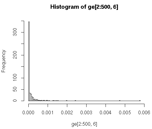
To bin a vector (break a list of numbers up into segments) and visualize the binning with a histogram:
> hist(ge[2:500,6],breaks=100,plot="True")  # what numbers are being binned here?  Try str(ge)
# see result below
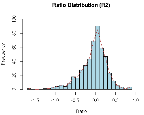
To draw a histogram of a data vector and spline the distribution curve, using the file cybert-allgene.txt (Copy the link location, then wget it to your HPC dir)
In another bash shell (open another terminal session or use byobu)
# take a look at it with 'head'
bash $ head cybert-allgene.txt  # try it, it's not pretty

bash $ cols cybert-allgene.txt |less -S  # try it, scroll with arrows;

# now switch back to the R session

> bth <- read.table(file=" cybert-allgene.txt",header=TRUE,sep="\t",comment.char="#")

# hmm - why didn't that work?  Oh yes, included an extra leading space.

> bth <- read.table(file="cybert-allgene.txt",header=TRUE,sep="\t",comment.char="#")

# better.  Now check it

> str(bth)
'data.frame':   500 obs. of  21 variables:
 $ L         : Factor w/ 500 levels "GH01001","GH01027",..: 416 491 67 462 452 409 253 257 191 309 ...
 $ R1        : num  -0.673 NA 0.152 -0.596 1.526 ...
 $ R2        : num  -0.37 -0.7 -0.743 -0.455 -0.238 ...
 $ R3        : num  -0.272 -0.467 -0.833 -0.343 1.413 ...
 $ R4        : num  -1.705 -1.679 -1.167 -0.376 0.362 ...
 $ R5        : num  -0.657 -0.962 -0.376 -0.289 0.698 ...
 $ ExprEst   : num  -0.111 NA -0.0364 0.0229 0.0921 ...
 $ nR        : int  5 4 5 5 5 5 5 5 5 4 ...
 $ meanR     : num  -0.735 -0.952 -0.593 -0.412 0.752 ...
 $ stdR      : num  0.57 0.525 0.503 0.119 0.737 ...
 $ rasdR     : num  0.306 0.491 0.282 0.308 0.425 ...
 $ bayesSD   : num  0.414 0.519 0.373 0.278 0.553 ...
 $ ttest     : num  -3.97 -3.67 -3.56 -3.31 3.04 ...
 $ bayesDF   : int  13 12 13 13 13 13 13 13 13 12 ...
 $ pVal      : num  0.00161 0.00321 0.00349 0.00566 0.00949 ...
 $ cum.ppde.p: num  0.0664 0.1006 0.1055 0.1388 0.1826 ...
 $ ppde.p    : num  0.105 0.156 0.163 0.209 0.266 ...
 $ ROC.x     : num  0.00161 0.00321 0.00349 0.00566 0.00949 ...
 $ ROC.y     : num  0.000559 0.001756 0.002009 0.004458 0.010351 ...
 $ Bonferroni: num  0.805 1 1 1 1 ...
 $ BH        : num  0.581 0.581 0.581 0.681 0.681 ...

# Create a histogram for the 'R2' column.  The following cmd not only plots the histogram
# but also populates the 'hhde' histogram object.
# breaks =  how many bins there should be (controls the size of the bins
# plot = to plot or not to plot
# labels = if T, each bar is labeled with the numeric value
# main, xlab, ylab = plot title, axis labels
# col = color of hist bars
# ylim, xlim = axis limits; if not set, the limits will be those of the data.

> hhde <-hist(bth$R2,breaks=30,plot="True",labels=F, main="Ratio Distribution (R2)",xlab="Ratio",ylab="Frequency", col="lightblue",ylim=c(0,100), xlim=c(-1.7,1.0))

# now plot a smoothed distribution using the hhde$mids (x) and hhde$counts (y)
# df = degrees of freedom, how much smoothing is applied;
#    (how closely the line will follow the values)
> lines(smooth.spline(hhde$mids,hhde$counts, df=20), lty=1, col = "brown")
16. Basic Statistics
Now (finally) let’s get some basic descriptive stats out of the original table. 1st, load the lib that has the functions we’ll need
> library(pastecs)  # load the lib that has the correct functions

> attach(ge) # make the C1.1 & C1.0 columns usable as variables.

# following line combines an R data structure by column.
# type 'help(cbind)' or '?cbind' for more info on cbind, rbind

> c1all <- cbind(C1.1,C1.0)

# the following calculates a table of descriptive stats for both the C1.1 & C1.0 variables
> stat.desc(c1all)
                      C1.1         C1.0
nbr.val       5.980000e+02 5.980000e+02
nbr.null      3.090000e+02 3.150000e+02
nbr.na        0.000000e+00 0.000000e+00
min          -3.363966e-02 0.000000e+00
max           0.000000e+00 1.832408e-02
range         3.363966e-02 1.832408e-02
sum          -1.787378e-01 8.965868e-02
median        0.000000e+00 0.000000e+00
mean         -2.988927e-04 1.499309e-04
SE.mean       6.688562e-05 3.576294e-05
CI.mean.0.95  1.313597e-04 7.023646e-05
var           2.675265e-06 7.648346e-07
std.dev       1.635624e-03 8.745482e-04
coef.var     -5.472277e+00 5.833009e+00
You can also feed column numbers (as oppo to variable names) to stat.desc to generate similar results:
stat.desc(some_table[2:13])
             stress_ko_n1 stress_ko_n2 stress_ko_n3 stress_wt_n1 stress_wt_n2
nbr.val      3.555700e+04 3.555700e+04 3.555700e+04 3.555700e+04 3.555700e+04
nbr.null     0.000000e+00 0.000000e+00 0.000000e+00 0.000000e+00 0.000000e+00
nbr.na       0.000000e+00 0.000000e+00 0.000000e+00 0.000000e+00 0.000000e+00
min          1.013390e-04 1.041508e-04 1.003806e-04 1.013399e-04 1.014944e-04
max          2.729166e+04 2.704107e+04 2.697153e+04 2.664553e+04 2.650478e+04
range        2.729166e+04 2.704107e+04 2.697153e+04 2.664553e+04 2.650478e+04
sum          3.036592e+07 2.995104e+07 2.977157e+07 3.054361e+07 3.055979e+07
median       2.408813e+02 2.540591e+02 2.377578e+02 2.396799e+02 2.382967e+02
mean         8.540068e+02 8.423388e+02 8.372915e+02 8.590042e+02 8.594593e+02
SE.mean      8.750202e+00 8.608451e+00 8.599943e+00 8.810000e+00 8.711472e+00
CI.mean.0.95 1.715066e+01 1.687283e+01 1.685615e+01 1.726787e+01 1.707475e+01
var          2.722458e+06 2.634967e+06 2.629761e+06 2.759796e+06 2.698411e+06
std.dev      1.649987e+03 1.623258e+03 1.621654e+03 1.661263e+03 1.642684e+03
coef.var     1.932054e+00 1.927085e+00 1.936785e+00 1.933941e+00 1.911300e+00

<etc>
There is also a basic function called summary, which will give summary stats on all components of a dataframe.
> summary(ge)
> summary(ge)
       b                gene            EC           C1.0
 b0001  :  1   0          : 20   0       :279   Min.   :0.000e+00
 b0002  :  1   0.000152968:  1   1.10.3.-:  4   1st Qu.:0.000e+00
 b0003  :  1   0.000158799:  1   2.7.7.7 :  4   Median :0.000e+00
 b0004  :  1   3.32E-06   :  1   5.2.1.8 :  4   Mean   :1.499e-04
 b0005  :  1   3.44E-05   :  1   5.-.-.- :  3   3rd Qu.:7.375e-05
 b0006  :  1   6.66E-05   :  1   1.-.-.- :  2   Max.   :1.832e-02
 (Other):592   (Other)    :573   (Other) :302
      C1.1                 C2.0                C2.1
 Min.   :-0.0336397   Min.   :0.0000000   Min.   :0.000e+00
 1st Qu.:-0.0001710   1st Qu.:0.0000000   1st Qu.:0.000e+00
 Median : 0.0000000   Median :0.0000000   Median :0.000e+00
 Mean   :-0.0002989   Mean   :0.0001423   Mean   :1.423e-04
 3rd Qu.: 0.0000000   3rd Qu.:0.0000754   3rd Qu.:5.927e-05
 Max.   : 0.0000000   Max.   :0.0149861   Max.   :1.462e-02

 [ rest of output trimmed ]
This is only the very beginning of what you can do with R. We’ve not even touched on the Bioconductor suite, which is one of the best known and supported tools to deal with Bioinformatics.
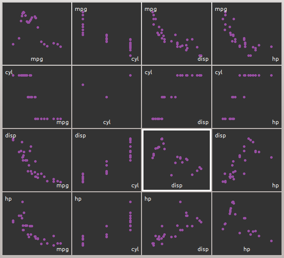
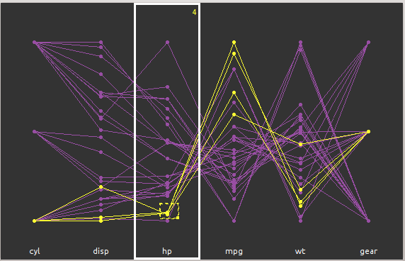
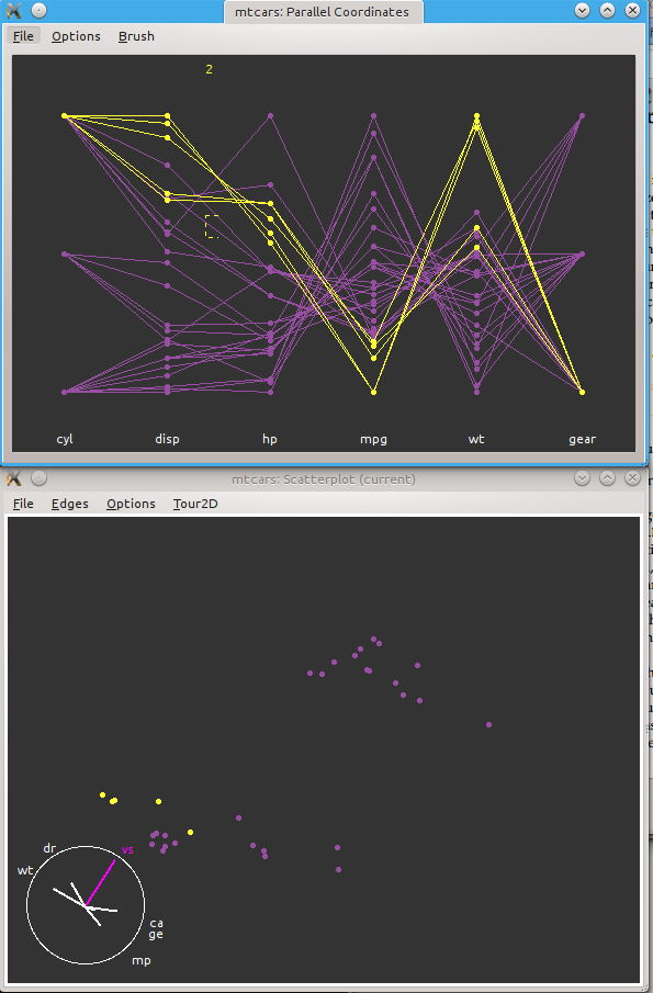
17. Visualizing Data with ggobi
While there are many ways in R to plot your data, one unique benefit that R provides is its interface to ggobi, an advanced visualization tool for multivariate data, which for the sake of argument is more than 3 variables.
rggobi takes an R dataframe and presents the variables in a very sophisticated way in realtime 3D, allowing you to visualize multiple variables in multiple ways.
> library("rggobi")  # load the library
> g <- ggobi(ge)     # R dataframe -> a ggobi object, and starts ggobi with that object

# were going to use the 'mtcars' data set which is a bunch of car data.
> g <- ggobi(mtcars)

# Now you have access to the entire ggobi interface via point and click (tho there are still a lot of choices and not all of them are straightforward)
18. Exporting Data
Ok, you’ve imported your data, analyzed it, generated some nice plots and dataframes. How do you export it to a file so it can be read by other applications? As you might expect, R provides some excellent documentation for this as well. The previously noted document R Data Import/Export describes it well. It’s definitely worthwhile reading it in full, but the very short version is that the most frequently used export function is to write dataframes into tabular files, essentially the reverse of reading Excel spreadsheets, but in text form. For this, we most often use the write.table() function. Using the ge dataframe already created, let’s output some of it:
> ge[1:3,] # lets see what it looks like 'raw'
      b             gene              EC        C1.0         C1.1        C2.0
1 b0001             thrL     0.000423101 0.000465440 -0.000858524 0.000433869
2 b0002 thrA+thrA1+thrA2 1.1.1.3+2.7.2.4 0.001018277 -0.002536156 0.001312524
3 b0003             thrB        2.7.1.39 0.000517967 -0.000915210 0.000582354
         C2.1        C3.0        C3.1        E1.0        E1.1        E2.0
1 0.000250998 0.000268929 0.000369315 0.000736700 0.000712840 0.000638379
2 0.001398845 0.000780489 0.000722073 0.001087711 0.001453382 0.002137451
3 0.000640462 0.000374730 0.000409490 0.000437738 0.000559135 0.000893933
         E2.1        E3.0        E3.1      C1.1Neg
1 0.000475292 0.000477763 0.000509705 -0.000429262
2 0.002153896 0.001605332 0.001626144 -0.001268078
3 0.000839385 0.000621375 0.000638264 -0.000457605


> write.table(ge[1:3,])

"b" "gene" "EC" "C1.0" "C1.1" "C2.0" "C2.1" "C3.0" "C3.1" "E1.0" "E1.1" "E2.0" "E2.1" "E3.0" "E3.1" "C1.1Neg"
"1" "b0001" "thrL" "0.000423101" 0.00046544 -0.000858524 0.000433869 0.000250998 0.000268929 0.000369315 0.0007367 0.00071284 0.000638379 0.000475292 0.000477763 0.000509705 -0.000429262
"2" "b0002" "thrA+thrA1+thrA2" "1.1.1.3+2.7.2.4" 0.001018277 -0.002536156 0.001312524 0.001398845 0.000780489 0.000722073 0.001087711 0.001453382 0.002137451 0.002153896 0.001605332 0.001626144 -0.001268078
"3" "b0003" "thrB" "2.7.1.39" 0.000517967 -0.00091521 0.000582354 0.000640462 0.00037473 0.00040949 0.000437738 0.000559135 0.000893933 0.000839385 0.000621375 0.000638264 -0.000457605

# in the write.table() format above, it's different due to the quoting and spacing.
# You can address all these in the various arguments to write.table(), for example:

> write.table(ge[1:3,], quote = FALSE, sep = "\t",row.names = FALSE,col.names = TRUE)
b       gene    EC      C1.0    C1.1    C2.0    C2.1    C3.0    C3.1    E1.0    E1.1    E2.0  E2.1     E3.0    E3.1    C1.1Neg
b0001   thrL    0.000423101     0.00046544      -0.000858524    0.000433869     0.000250998   0.000268929      0.000369315     0.0007367       0.00071284      0.000638379     0.000475292   0.000477763      0.000509705     -0.000429262
b0002   thrA+thrA1+thrA2        1.1.1.3+2.7.2.4 0.001018277     -0.002536156    0.001312524   0.001398845      0.000780489     0.000722073     0.001087711     0.001453382     0.002137451   0.002153896      0.001605332     0.001626144     -0.001268078
b0003   thrB    2.7.1.39        0.000517967     -0.00091521     0.000582354     0.000640462   0.00037473       0.00040949      0.000437738     0.000559135     0.000893933     0.000839385   0.000621375      0.000638264     -0.000457605


# note that I omitted a file specification to dump the output to the screen.  To send
# the same output to a file, you just have to specify it:

> write.table(ge[1:3,], file="/path/to/the/file.txt", quote = FALSE, sep = "\t",row.names = FALSE,col.names = TRUE)


# play around with the arguments, reversing or modifying the argument values.
# the entire documentation for write.table is available from the commandline with
# '?write.table'
19. The commercial Revolution R is free to Academics
Recently a company called Revolution Analytics has started to commercialize R, smoothing off the rough edges, providing a GUI, improving the memory management, speeding up some core routines. This commercial version is available free to academics via a single user license (and therefore it cannot be made available on the BDUC cluster). If you’re interested in it, you can download it from here.
20. Resources
20.1. Introduction to Linux
-
The An Introduction to the HPC Computing Facility aka The HPC User’s HOWTO.
-
The BioLinux - a gentle introduction to Bioinformatics on Linux class slides:
-
the topical Biostars StackExchange Resource
-
the SeqAnswer list
-
Instructors:
-
Jenny Wu <jiew5@uci.edu>
-
Harry Mangalam <harry.mangalam@uciedu>
-
21. Other R Resources
If local help is not installed, most R help can be found in PDF and HTML at the R documentation page.
21.1. Local Lightweight Introductions to R
21.2. External Introductions to R
There is a very useful 100 page PDF book called: An Introduction to R (also in HTML). Especially note Chapter 1 and Appendix A on page 78, which is a more sophisticated, (but less gentle) tutorial than this.
Note also that if you have experience in SAS or SPSS, there is a good introduction written especially with this experience in mind. It has been expanded into a large book (to be released imminently), but much of the core is still available for free as R for SAS and SPSS Users
There is another nice Web page that provides a quick, broad intro to R appropriately called Using R for psychological research: A simple guide to an elegant package which manages to compress a great deal of what you need to know about R into about 30 screens of well-cross-linked HTML.
There is also a website that expands on simple tutorials and examples, so after buzzing thru this very simple example, please continue to the QuickR website
Thomas Girke at UC Riverside has a very nice HTML Introduction to R and Bioconductor as part of his Bioinformatics Core, which also runs frequent R-related courses which may be of interest for the Southern California area.
22. Distribution & Release Conditions
If this Document has been sent to you as a file instead of as a link, some of the content may be lost. The original page is here. The AsciiDoc source is here, which has embedded comments that show how to convert the source to the HTML. AsciiDoc is a simple and simply fantastic documentation language - thanks to Stuart Rackham for developing it.

This work is licensed under a Creative Commons Attribution-ShareAlike 3.0 Unported License.